A more complex compositional model

This example sets up a more complex compositional simulation with five different components. Other than that, the example is similar to the others that include wells and is therefore not commented in great detail.

using MultiComponentFlash

n2_ch4 = MolecularProperty(0.0161594, 4.58e6, 189.515, 9.9701e-05, 0.00854)
co2 = MolecularProperty(0.04401, 7.3866e6, 304.200, 9.2634e-05, 0.228)
c2_5 = MolecularProperty(0.0455725, 4.0955e6, 387.607, 2.1708e-04, 0.16733)
c6_13 = MolecularProperty(0.117740, 3.345e6, 597.497, 3.8116e-04, 0.38609)
c14_24 = MolecularProperty(0.248827, 1.768e6, 698.515, 7.2141e-04, 0.80784)

bic = [0.11883 0.00070981 0.00077754 0.01 0.011;
       0.00070981 0.15 0.15 0.15 0.15;
       0.00077754 0.15 0 0 0;
       0.01 0.15 0 0 0;
       0.011 0.15 0 0 0]

mixture = MultiComponentMixture([n2_ch4, co2, c2_5, c6_13, c14_24], A_ij = bic, names = ["N2-CH4", "CO2", "C2-5", "C6-13", "C14-24"])
eos = GenericCubicEOS(mixture, PengRobinson())

using Jutul, JutulDarcy, CairoMakie
Darcy, bar, kg, meter, Kelvin, day = si_units(:darcy, :bar, :kilogram, :meter, :Kelvin, :day)
nx = ny = 20
nz = 2

dims = (nx, ny, nz)
g = CartesianMesh(dims, (1000.0, 1000.0, 1.0))
nc = number_of_cells(g)
K = repeat([0.05*Darcy], 1, nc)
res = reservoir_domain(g, porosity = 0.25, permeability = K)

DataDomain wrapping CartesianMesh (3D) with 20x20x2=800 cells with 17 data fields added:
  800 Cells
    :permeability => 1×800 Matrix{Float64}
    :porosity => 800 Vector{Float64}
    :rock_thermal_conductivity => 800 Vector{Float64}
    :fluid_thermal_conductivity => 800 Vector{Float64}
    :rock_density => 800 Vector{Float64}
    :cell_centroids => 3×800 Matrix{Float64}
    :volumes => 800 Vector{Float64}
  1920 Faces
    :neighbors => 2×1920 Matrix{Int64}
    :areas => 1920 Vector{Float64}
    :normals => 3×1920 Matrix{Float64}
    :face_centroids => 3×1920 Matrix{Float64}
  3840 HalfFaces
    :half_face_cells => 3840 Vector{Int64}
    :half_face_faces => 3840 Vector{Int64}
  960 BoundaryFaces
    :boundary_areas => 960 Vector{Float64}
    :boundary_centroids => 3×960 Matrix{Float64}
    :boundary_normals => 3×960 Matrix{Float64}
    :boundary_neighbors => 960 Vector{Int64}

Set up a vertical well in the first corner, perforated in all layers

prod = setup_vertical_well(g, K, nx, ny, name = :Producer)

MultiSegmentWell [Producer] (3 nodes, 2 segments, 2 perforations)

Set up an injector in the opposite corner, perforated in all layers

inj = setup_vertical_well(g, K, 1, 1, name = :Injector)

rhoLS = 1000.0*kg/meter^3
rhoVS = 100.0*kg/meter^3

rhoS = [rhoLS, rhoVS]
L, V = LiquidPhase(), VaporPhase()

(LiquidPhase(), VaporPhase())

Define system and realize on grid

sys = MultiPhaseCompositionalSystemLV(eos, (L, V))
model, parameters = setup_reservoir_model(res, sys, wells = [inj, prod], reference_densities = rhoS, block_backend = true);
kr = BrooksCoreyRelativePermeabilities(sys, 2.0, 0.0, 1.0)
model = replace_variables!(model, RelativePermeabilities = kr)

push!(model[:Reservoir].output_variables, :Saturations)

parameters[:Reservoir][:Temperature] = 387.45*Kelvin
state0 = setup_reservoir_state(model, Pressure = 225*bar, OverallMoleFractions = [0.463, 0.01640, 0.20520, 0.19108, 0.12432]);

dt = repeat([2.0]*day, 365)
rate_target = TotalRateTarget(0.0015)
I_ctrl = InjectorControl(rate_target, [0, 1, 0, 0, 0], density = rhoVS)
bhp_target = BottomHolePressureTarget(100*bar)
P_ctrl = ProducerControl(bhp_target)

controls = Dict()
controls[:Injector] = I_ctrl
controls[:Producer] = P_ctrl
forces = setup_reservoir_forces(model, control = controls)
ws, states = simulate_reservoir(state0, model, dt, parameters = parameters, forces = forces)
#!

ReservoirSimResult with 365 entries:

  wells (2 present):
    :Producer
    :Injector
    Results per well:
       :Surface total rate => Vector{Float64} of size (365,)
       :Surface oil rate => Vector{Float64} of size (365,)
       :Bottom hole pressure => Vector{Float64} of size (365,)
       :Surface gas rate => Vector{Float64} of size (365,)
       :Surface liquid rate (water + oil) => Vector{Float64} of size (365,)
       :Total surface mass rate => Vector{Float64} of size (365,)

  states (Vector with 365 entries, reservoir variables for each state)
    :LiquidMassFractions => Matrix{Float64} of size (5, 800)
    :OverallMoleFractions => Matrix{Float64} of size (5, 800)
    :Saturations => Matrix{Float64} of size (2, 800)
    :Pressure => Vector{Float64} of size (800,)
    :VaporMassFractions => Matrix{Float64} of size (5, 800)
    :TotalMasses => Matrix{Float64} of size (5, 800)

  time (report time for each state)
     Vector{Float64} of length 365

  result (extended states, reports)
     SimResult with 365 entries

  extra
     Dict{Any, Any} with keys :simulator, :config

  Completed at Mar. 10 2024 20:03 after 40 seconds, 159 milliseconds, 651.6 microseconds.

Once the simulation is done, we can plot the states

sg = states[end][:OverallMoleFractions][2, :]
fig, ax, p = plot_cell_data(g, sg)
fig
#!
sg = states[end][:Saturations][2, :]
fig, ax, p = plot_cell_data(g, sg)
fig
#!
p = states[end][:Pressure]
fig, ax, p = plot_cell_data(g, p)
fig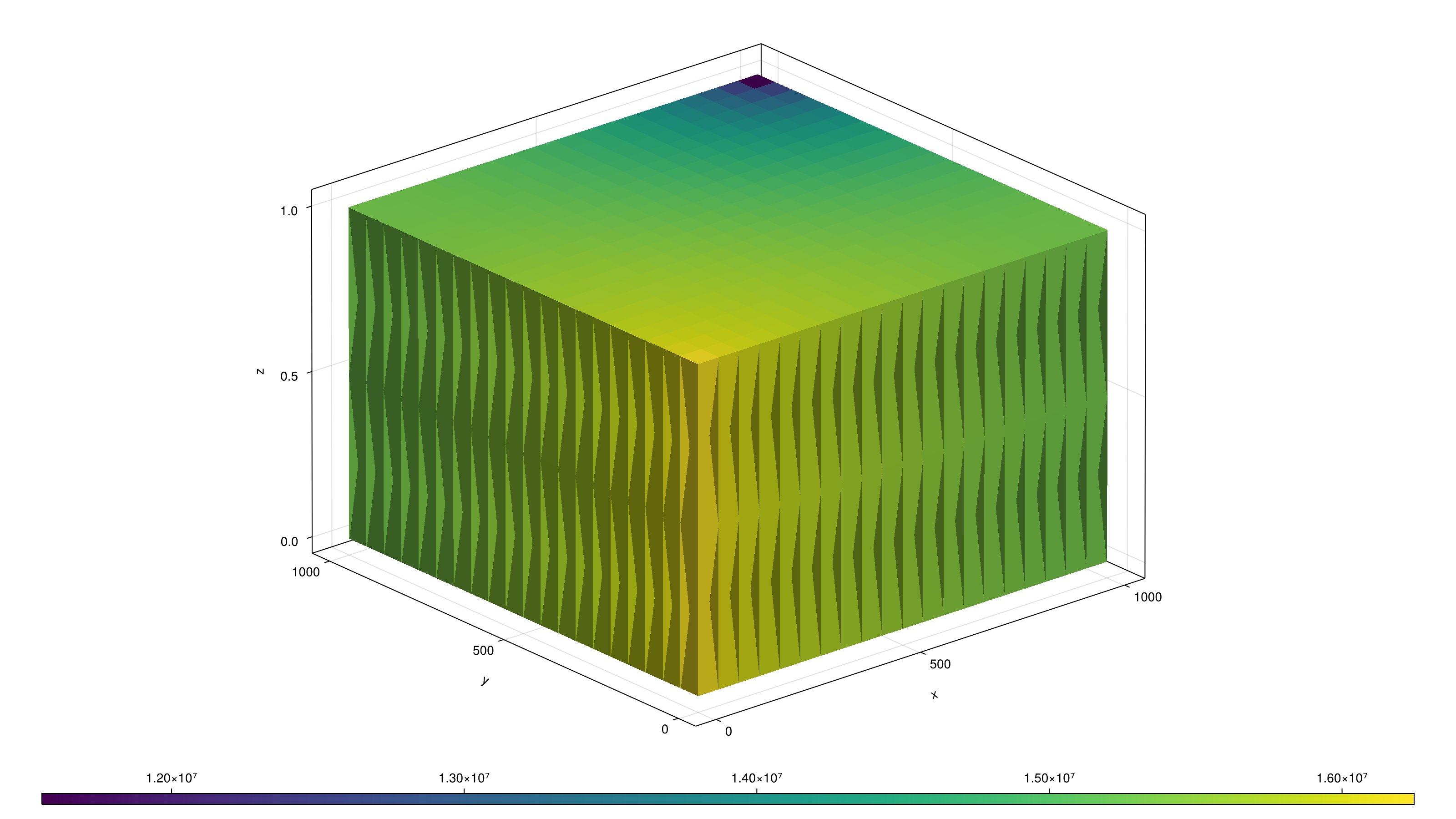

Example on GitHub

If you would like to run this example yourself, it can be downloaded from the JutulDarcy.jl GitHub repository.

This page was generated using Literate.jl.