Buckley-Leverett two-phase problem
The Buckley-Leverett test problem is a classical reservoir simulation benchmark that demonstrates the nonlinear displacement process of a viscous fluid being displaced by a less viscous fluid, typically taken to be water displacing oil.
Problem definition
This is a simple model without wells, where the flow is driven by a simple source term and a simple constant pressure boundary condition at the outlet. We define a function that sets up a two-phase system, a simple 1D domain and replaces the default relative permeability functions with quadratic functions:
$k_{r\alpha}(S) = \min \left(\frac{S - S_r}{1 - S_r}, 1\right)^n, S_r = 0.2, n = 2$
In addition, the phase viscosities are treated as constant parameters of 1 and 5 centipoise for the displacing and resident fluids, respectively.
The function is parametrized on the number of cells and the number of time-steps used to solve the model. This function, since it uses a relatively simple setup without wells, uses the Jutul functions directly.
using JutulDarcy, Jutul
function solve_bl(;nc = 100, time = 1.0, nstep = nc)
    T = time
    tstep = repeat([T/nstep], nstep)
    domain = get_1d_reservoir(nc)
    nc = number_of_cells(domain)
    timesteps = tstep*3600*24
    bar = 1e5
    p0 = 100*bar
    sys = ImmiscibleSystem((LiquidPhase(), VaporPhase()))
    model = SimulationModel(domain, sys)
    kr = BrooksCoreyRelativePermeabilities(sys, [2.0, 2.0], [0.2, 0.2])
    replace_variables!(model, RelativePermeabilities = kr)
    tot_time = sum(timesteps)
    pv = pore_volume(domain)
    irate = 500*sum(pv)/tot_time
    src  = SourceTerm(1, irate, fractional_flow = [1.0, 0.0])
    bc = FlowBoundaryCondition(nc, p0/2)
    forces = setup_forces(model, sources = src, bc = bc)
    parameters = setup_parameters(model, PhaseViscosities = [1e-3, 5e-3]) # 1 and 5 cP
    state0 = setup_state(model, Pressure = p0, Saturations = [0.0, 1.0])
    states, report = simulate(state0, model, timesteps,
        forces = forces, parameters = parameters, info_level = -1)
    return states, model, report
end
solve_bl (generic function with 1 method)Run the base case
We solve a small model with 100 cells and 100 steps to serve as the baseline.
n, n_f = 100, 1000
states, model, report = solve_bl(nc = n)
print_stats(report)
╭────────────────┬───────────┬───────────────┬──────────┬──────────╮
│ Iteration type │ Avg/step │ Avg/ministep │ Time per │ Total │
│ │ 100 steps │ 100 ministeps │ ms │ (wasted) │
├────────────────┼───────────┼───────────────┼──────────┼──────────┤
│ Newton │ 3.31 │ 3.31 │ 2.0080 │ 331 (0) │
│ Linearization │ 4.31 │ 4.31 │ 1.5421 │ 431 (0) │
│ Linear solver │ 3.31 │ 3.31 │ 2.0080 │ 331 (0) │
╰────────────────┴───────────┴───────────────┴──────────┴──────────╯
╭────────────────┬────────┬────────────┬──────────╮
│ Timing type │ Each │ Relative │ Total │
│ │ ms │ Percentage │ ms │
├────────────────┼────────┼────────────┼──────────┤
│ Properties │ 0.0123 │ 0.61 % │ 4.0666 │
│ Equations │ 0.3781 │ 24.52 % │ 162.9474 │
│ Assembly │ 0.0065 │ 0.42 % │ 2.7825 │
│ Linear solve │ 0.1812 │ 9.02 % │ 59.9691 │
│ Preconditioner │ 0.0000 │ 0.00 % │ 0.0000 │
│ Update │ 0.0107 │ 0.53 % │ 3.5546 │
│ Convergence │ 0.0114 │ 0.74 % │ 4.9200 │
│ Input/Output │ 0.1881 │ 2.83 % │ 18.8110 │
│ Other │ 1.2314 │ 61.32 % │ 407.5880 │
├────────────────┼────────┼────────────┼──────────┤
│ Total │ 2.0080 │ 100.00 % │ 664.6390 │
╰────────────────┴────────┴────────────┴──────────╯Run refined version (1000 cells, 1000 steps)
Using a grid with 100 cells will not yield a fully converged solution. We can increase the number of cells at the cost of increasing the runtime a bit. Note that most of the time is spent in the linear solver, which uses a direct sparse LU factorization by default. For larger problems it is recommended to use an iterative solver.
states_refined, _, report_refined = solve_bl(nc = n_f);
print_stats(report_refined)
╭────────────────┬────────────┬────────────────┬──────────┬──────────╮
│ Iteration type │ Avg/step │ Avg/ministep │ Time per │ Total │
│ │ 1000 steps │ 1000 ministeps │ ms │ (wasted) │
├────────────────┼────────────┼────────────────┼──────────┼──────────┤
│ Newton │ 3.265 │ 3.265 │ 2.0837 │ 3265 (0) │
│ Linearization │ 4.265 │ 4.265 │ 1.5951 │ 4265 (0) │
│ Linear solver │ 3.265 │ 3.265 │ 2.0837 │ 3265 (0) │
╰────────────────┴────────────┴────────────────┴──────────┴──────────╯
╭────────────────┬────────┬────────────┬────────╮
│ Timing type │ Each │ Relative │ Total │
│ │ ms │ Percentage │ s │
├────────────────┼────────┼────────────┼────────┤
│ Properties │ 0.0673 │ 3.23 % │ 0.2198 │
│ Equations │ 0.0517 │ 3.24 % │ 0.2203 │
│ Assembly │ 0.0484 │ 3.03 % │ 0.2064 │
│ Linear solve │ 1.7484 │ 83.91 % │ 5.7085 │
│ Preconditioner │ 0.0000 │ 0.00 % │ 0.0000 │
│ Update │ 0.0235 │ 1.13 % │ 0.0767 │
│ Convergence │ 0.0160 │ 1.00 % │ 0.0682 │
│ Input/Output │ 0.2019 │ 2.97 % │ 0.2019 │
│ Other │ 0.0311 │ 1.49 % │ 0.1014 │
├────────────────┼────────┼────────────┼────────┤
│ Total │ 2.0837 │ 100.00 % │ 6.8032 │
╰────────────────┴────────┴────────────┴────────╯Plot results
We plot the saturation front for the base case at different times together with the final solution for the refined model. In this case, refining the grid by a factor 10 gave us significantly less smearing of the trailing front.
using CairoMakie
x = range(0, stop = 1, length = n)
x_f = range(0, stop = 1, length = n_f)
f = Figure()
ax = Axis(f[1, 1], ylabel = "Saturation", title = "Buckley-Leverett")
for i in 1:6:length(states)
    lines!(ax, x, states[i][:Saturations][1, :], color = :darkgray)
end
lines!(ax, x_f, states_refined[end][:Saturations][1, :], color = :red)
f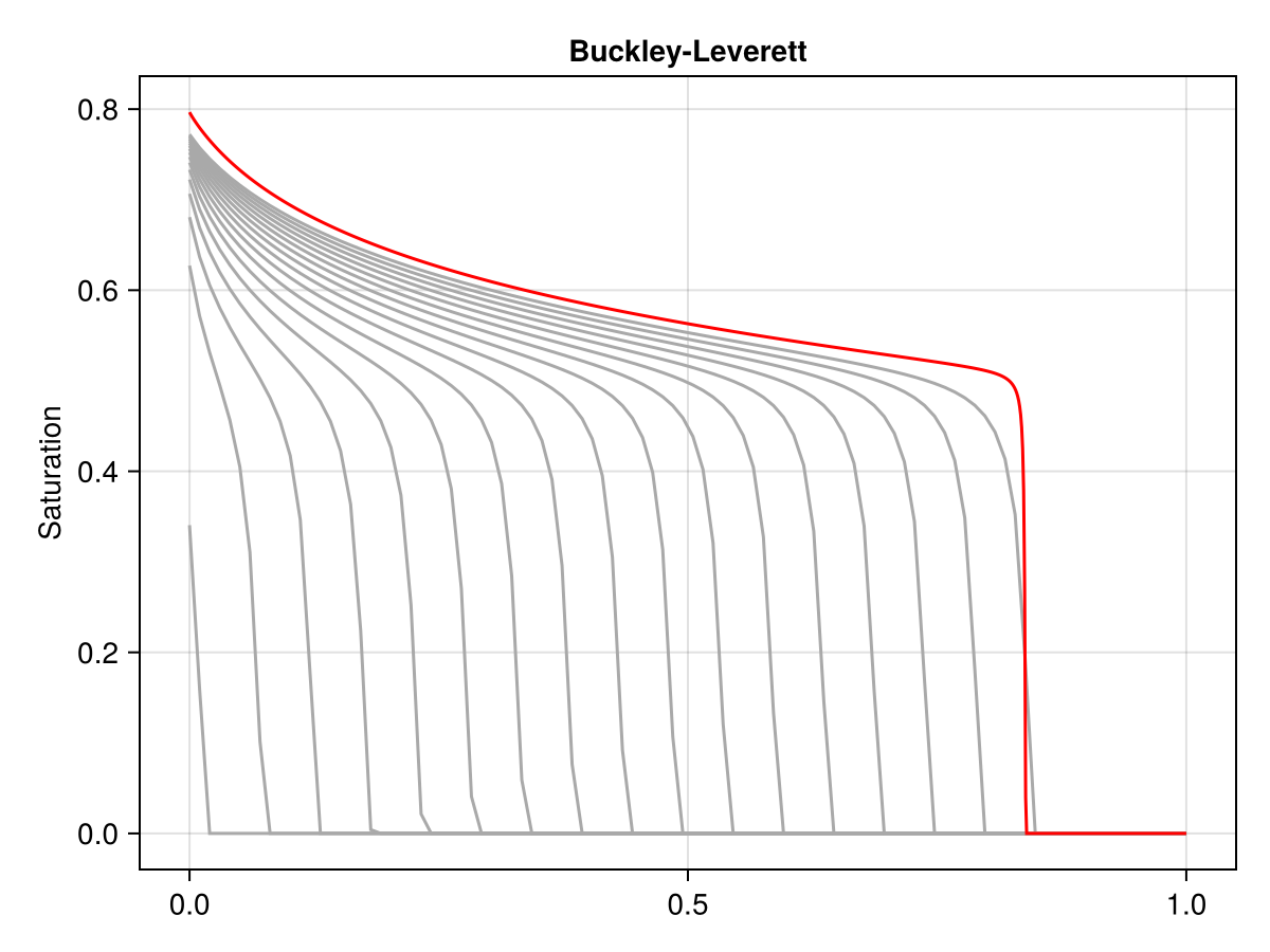
Example on GitHub
If you would like to run this example yourself, it can be downloaded from the JutulDarcy.jl GitHub repository.
This page was generated using Literate.jl.