using Jutul
using JutulDarcy
using LinearAlgebra
using CairoMakie
Example demonstrating optimzation of parameters against observations
We create a simple test problem: A 1D nonlinear displacement. The observations are generated by solving the same problem with the true parameters. We then match the parameters against the observations using a different starting guess for the parameters, but otherwise the same physical description of the system.
function setup_bl(;nc = 100, time = 1.0, nstep = 100, poro = 0.1, perm = 9.8692e-14)
    T = time
    tstep = repeat([T/nstep], nstep)
    G = get_1d_reservoir(nc, poro = poro, perm = perm)
    nc = number_of_cells(G)

    bar = 1e5
    p0 = 1000*bar
    sys = ImmiscibleSystem((LiquidPhase(), VaporPhase()))
    model = SimulationModel(G, sys)
    model.primary_variables[:Pressure] = Pressure(minimum = -Inf, max_rel = nothing)
    kr = BrooksCoreyRelativePermeabilities(sys, [2.0, 2.0])
    replace_variables!(model, RelativePermeabilities = kr)
    tot_time = sum(tstep)

    parameters = setup_parameters(model, PhaseViscosities = [1e-3, 5e-3]) # 1 and 5 cP
    state0 = setup_state(model, Pressure = p0, Saturations = [0.0, 1.0])

    irate = 100*sum(parameters[:FluidVolume])/tot_time
    src  = [SourceTerm(1, irate, fractional_flow = [1.0-1e-3, 1e-3]),
            SourceTerm(nc, -irate, fractional_flow = [1.0, 0.0])]
    forces = setup_forces(model, sources = src)

    return (model, state0, parameters, forces, tstep)
end
setup_bl (generic function with 1 method)Number of cells and time-steps
N = 100
Nt = 100
poro_ref = 0.1
perm_ref = 9.8692e-149.8692e-14Set up and simulate reference
model_ref, state0_ref, parameters_ref, forces, tstep = setup_bl(nc = N, nstep = Nt, poro = poro_ref, perm = perm_ref)
states_ref, = simulate(state0_ref, model_ref, tstep, parameters = parameters_ref, forces = forces, info_level = -1)
SimResult with 100 entries:
states (model variables)
:Saturations => Matrix{Float64} of size (2, 100)
:Pressure => Vector{Float64} of size (100,)
:TotalMasses => Matrix{Float64} of size (2, 100)
reports (timing/debug information)
:ministeps => Vector{Any} of size (1,)
:total_time => Float64
:output_time => Float64
Completed at Mar. 10 2024 20:03 after 3 seconds, 247 milliseconds, 378.7 microseconds.Set up another case where the porosity is different
model, state0, parameters, = setup_bl(nc = N, nstep = Nt, poro = 2*poro_ref, perm = 1.0*perm_ref)
states, rep = simulate(state0, model, tstep, parameters = parameters, forces = forces, info_level = -1)
SimResult with 100 entries:
states (model variables)
:Saturations => Matrix{Float64} of size (2, 100)
:Pressure => Vector{Float64} of size (100,)
:TotalMasses => Matrix{Float64} of size (2, 100)
reports (timing/debug information)
:ministeps => Vector{Any} of size (1,)
:total_time => Float64
:output_time => Float64
Completed at Mar. 10 2024 20:03 after 32 milliseconds, 375 microseconds, 417 nanoseconds.Plot the results
fig = Figure()
ax = Axis(fig[1, 1], title = "Saturation")
lines!(ax, states_ref[end][:Saturations][1, :], label = "Reference")
lines!(ax, states[end][:Saturations][1, :], label = "Initial guess")
axislegend(ax)
ax = Axis(fig[1, 2], title = "Pressure")
lines!(ax, states_ref[end][:Pressure], label = "Reference")
lines!(ax, states[end][:Pressure], label = "Initial guess")
axislegend(ax)
fig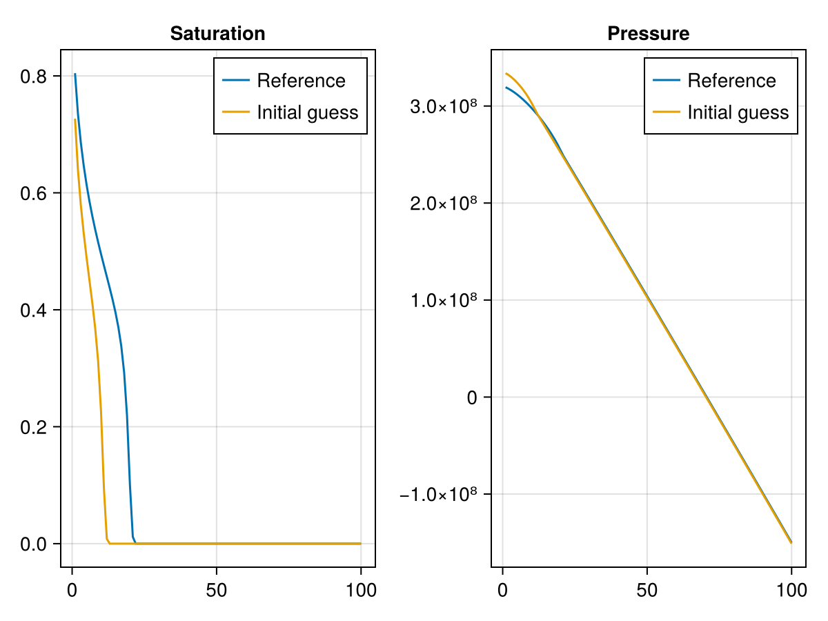
Define objective function
Define objective as mismatch between water saturation in current state and reference state. The objective function is currently a sum over all time steps. We implement a function for one term of this sum.
function mass_mismatch(m, state, dt, step_no, forces)
    state_ref = states_ref[step_no]
    fld = :Saturations
    val = state[fld]
    ref = state_ref[fld]
    err = 0
    for i in axes(val, 2)
        err += (val[1, i] - ref[1, i])^2
    end
    return dt*err
end
@assert Jutul.evaluate_objective(mass_mismatch, model, states_ref, tstep, forces) == 0.0
@assert Jutul.evaluate_objective(mass_mismatch, model, states, tstep, forces) > 0.0
Set up a configuration for the optimization. This by default enables all parameters for
optimization, with relative box limits 0.1 and 10 specified here. If use_scaling is enabled the variables in the optimization are scaled so that their actual limits are approximately box limits.
We are not interested in matching gravity effects or viscosity here. Transmissibilities are derived from permeability and varies significantly. We can set log scaling to get a better conditioned optimization system, without changing the limits or the result.
cfg = optimization_config(model, parameters, use_scaling = true, rel_min = 0.1, rel_max = 10)
for (ki, vi) in cfg
    if ki in [:TwoPointGravityDifference, :PhaseViscosities]
        vi[:active] = false
    end
    if ki == :Transmissibilities
        vi[:scaler] = :log
    end
end
print_obj = 100100Set up parameter optimization.
This gives us a set of function handles together with initial guess and limits. Generally calling either of the functions will mutate the data Dict. The options are: Fo(x) -> evaluate objective dFo(dFdx, x) -> evaluate gradient of objective, mutating dFdx (may trigger evaluation of Fo) Fand_dF(F, dFdx, x) -> evaluate F and/or dF. Value of nothing will mean that the corresponding entry is skipped.
F_o, dF_o, F_and_dF, x0, lims, data = setup_parameter_optimization(model, state0, parameters, tstep, forces, mass_mismatch, cfg, print = print_obj, param_obj = true);
F_initial = F_o(x0)
dF_initial = dF_o(similar(x0), x0)
@info "Initial objective: $F_initial, gradient norm $(norm(dF_initial))"
Parameters for model
┌────────────────────┬────────┬─────┬─────────┬─────────────────┬─────────────┬──────────────────────┬─────────┐
│ Name │ Entity │ N │ Scale │ Abs. limits │ Rel. limits │ Limits │ Lumping │
├────────────────────┼────────┼─────┼─────────┼─────────────────┼─────────────┼──────────────────────┼─────────┤
│ Transmissibilities │ Faces │ 99 │ log │ [0, Inf] │ [0.1, 10] │ [9.87e-13, 9.87e-11] │ - │
│ FluidVolume │ Cells │ 100 │ default │ [2.22e-16, Inf] │ [0.1, 10] │ [0.0002, 0.02] │ - │
└────────────────────┴────────┴─────┴─────────┴─────────────────┴─────────────┴──────────────────────┴─────────┘
[ Info: Initial objective: 0.6770524183270709, gradient norm 4.12674840425729Link to an optimizer package
We use Optim.jl but the interface is general enough that e.g. LBFGSB.jl can easily be swapped in.
LBFGS is a good choice for this problem, as Jutul provides sensitivities via adjoints that are inexpensive to compute.
using Optim
lower, upper = lims
inner_optimizer = LBFGS()
opts = Optim.Options(store_trace = true, show_trace = true, time_limit = 30)
results = optimize(Optim.only_fg!(F_and_dF), lower, upper, x0, Fminbox(inner_optimizer), opts)
x = results.minimizer
display(results)
F_final = F_o(x)3.0208590097000804e-5Compute the solution using the tuned parameters found in x.
parameters_t = deepcopy(parameters)
devectorize_variables!(parameters_t, model, x, data[:mapper], config = data[:config])
x_truth = vectorize_variables(model_ref, parameters_ref, data[:mapper], config = data[:config])

states_tuned, = simulate(state0, model, tstep, parameters = parameters_t, forces = forces, info_level = -1);
nothing
Plot final parameter spread
@info "Final residual $F_final (down from $F_initial)"
fig = Figure()
ax1 = Axis(fig[1, 1], title = "Scaled parameters", ylabel = "Value")
scatter!(ax1, x, label = "Final X")
scatter!(ax1, x0, label = "Initial X")
lines!(ax1, lower, label = "Lower bound")
lines!(ax1, upper, label = "Upper bound")
axislegend()
fig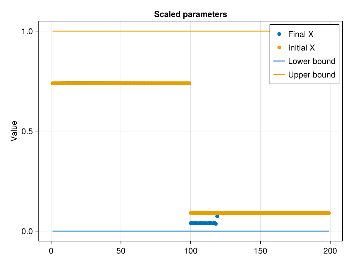
Plot the final solutions.
Note that we only match saturations - so any match in pressure is not guaranteed.
fig = Figure()
ax = Axis(fig[1, 1], title = "Saturation")
lines!(ax, states_ref[end][:Saturations][1, :], label = "Reference")
lines!(ax, states[end][:Saturations][1, :], label = "Initial guess")
lines!(ax, states_tuned[end][:Saturations][1, :], label = "Tuned")

axislegend(ax)
ax = Axis(fig[1, 2], title = "Pressure")
lines!(ax, states_ref[end][:Pressure], label = "Reference")
lines!(ax, states[end][:Pressure], label = "Initial guess")
lines!(ax, states_tuned[end][:Pressure], label = "Tuned")
axislegend(ax)
fig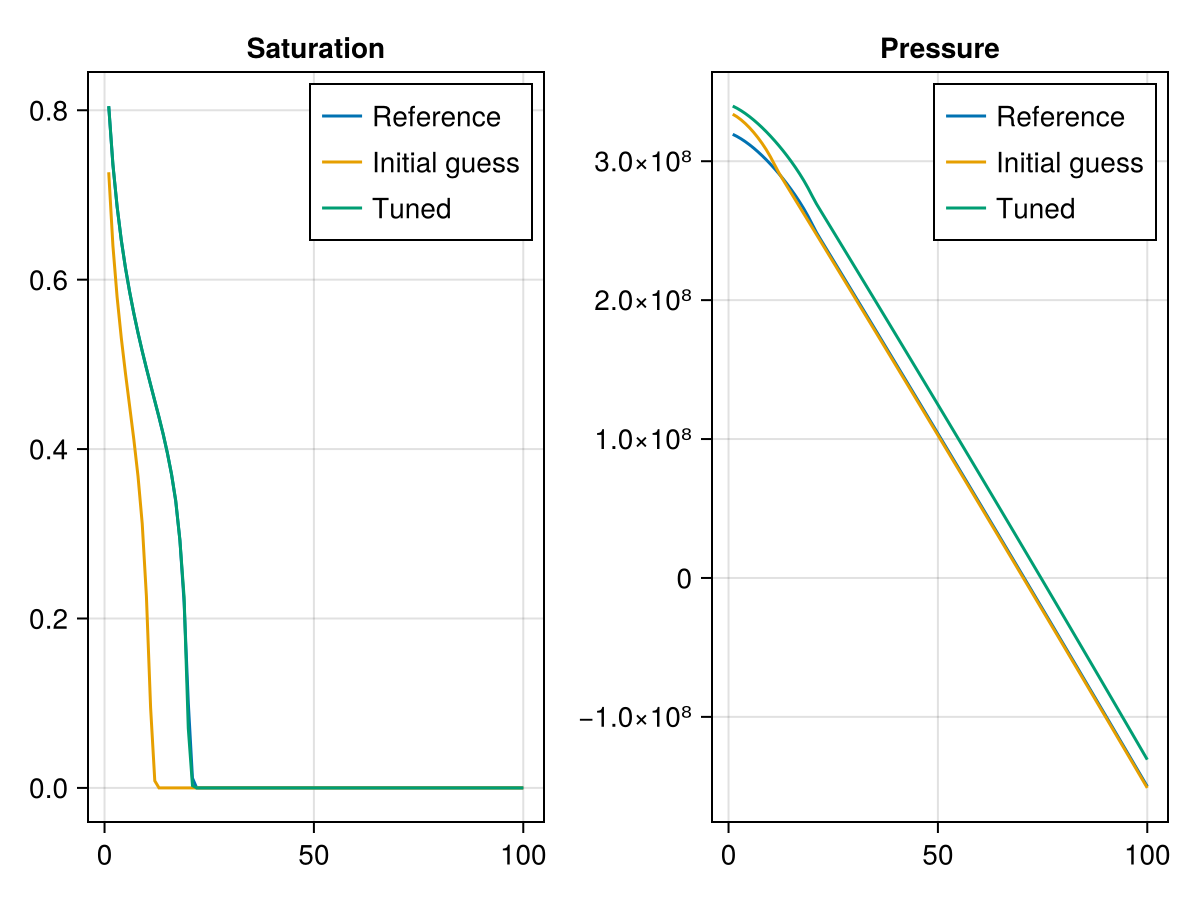
Plot the objective history and function evaluations
fig = Figure()
ax1 = Axis(fig[1, 1], yscale = log10, title = "Objective evaluations", xlabel = "Iterations", ylabel = "Objective")
plot!(ax1, data[:obj_hist][2:end])
ax2 = Axis(fig[1, 2], yscale = log10, title = "Outer optimizer", xlabel = "Iterations", ylabel = "Objective")
t = map(x -> x.value, Optim.trace(results))
plot!(ax2, t)
display(fig)
CairoMakie.Screen{IMAGE}
Example on GitHub
If you would like to run this example yourself, it can be downloaded from the JutulDarcy.jl GitHub repository.
This page was generated using Literate.jl.