Rank Histograms

Rank histograms and probability-integral-transform (PIT) histograms are diagnostic tools for checking whether an ensemble correctly represents the true distribution. A well-calibrated ensemble produces a uniform histogram.

This example demonstrates three approaches:

Gregory resampling — resample via the MLMC inverse-CDF, then compute ranks.
KDE CDF — estimate the CDF with kernel density estimation, then evaluate at truth.
MaxEnt CDF — estimate the CDF with maximum entropy, then evaluate at truth.

Model setup

We use a simple Gaussian model $X \sim \mathcal{N}(2,\, 0.5^2)$ with three levels that add decreasing amounts of noise.

using MultilevelMonteCarlo
using CairoMakie
using Statistics
using Random
Random.seed!(42)

μ_true = 2.0
σ_true = 0.5

levels = Function[
    params -> params + 0.2 * randn(),    # coarse — added noise σ = 0.2
    params -> params + 0.02 * randn(),   # medium — added noise σ = 0.02
    params -> Float64(params),           # fine   — exact
]

draw_parameters() = μ_true + σ_true * randn()
qoi_function = identity

samples_per_level = [2000, 1000, 200]

Gregory rank histogram

We run rank_histogram_gregory to collect ranks. Each iteration draws a truth sample from the finest level, builds a fresh MLMC ensemble, Gregory-resamples, and records where the truth falls in the sorted ensemble.

n_rank = 300
n_resamples = 500

ranks = rank_histogram_gregory(levels, qoi_function, draw_parameters,
                               n_rank, samples_per_level;
                               number_of_resamples = n_resamples)

A flat histogram indicates correct calibration:

fig = Figure(size = (700, 400))
ax = Axis(fig[1, 1];
    title  = "Gregory rank histogram",
    xlabel = "Rank",
    ylabel = "Count",
)
n_bins = 20
hist!(ax, Float64.(ranks); bins = n_bins, color = :steelblue, strokewidth = 1)
expected_per_bin = n_rank / n_bins
hlines!(ax, [expected_per_bin]; color = :red, linestyle = :dash,
        label = "Expected (uniform)")
axislegend(ax; position = :rt)

Gregory rank histogram

KDE PIT histogram

rank_histogram_cdf with estimate_cdf_mlmc_kernel_density produces PIT values that should be $\mathrm{Uniform}(0,1)$ if the KDE CDF is well calibrated.

pit_kde = rank_histogram_cdf(levels, qoi_function, draw_parameters,
                             n_rank, samples_per_level,
                             estimate_cdf_mlmc_kernel_density)

fig = Figure(size = (700, 400))
ax = Axis(fig[1, 1];
    title  = "PIT histogram — KDE CDF",
    xlabel = "PIT value",
    ylabel = "Count",
)
hist!(ax, pit_kde; bins = n_bins, color = :teal, strokewidth = 1)
expected_per_bin_cdf = n_rank / n_bins
hlines!(ax, [expected_per_bin_cdf]; color = :red, linestyle = :dash,
        label = "Expected (uniform)")
axislegend(ax; position = :rt)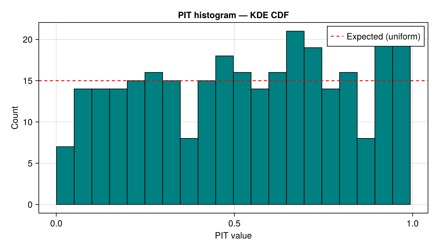

KDE PIT histogram

MaxEnt PIT histogram

Using estimate_cdf_maxent with $R = 6$ Legendre moments:

maxent_cdf(s, i) = first(estimate_cdf_maxent(s, i; R = 4))

pit_maxent = rank_histogram_cdf(levels, qoi_function, draw_parameters,
                                n_rank, samples_per_level,
                                maxent_cdf)

fig = Figure(size = (700, 400))
ax = Axis(fig[1, 1];
    title  = "PIT histogram — MaxEnt CDF",
    xlabel = "PIT value",
    ylabel = "Count",
)
hist!(ax, pit_maxent; bins = n_bins, color = :darkorange, strokewidth = 1)
hlines!(ax, [expected_per_bin_cdf]; color = :red, linestyle = :dash,
        label = "Expected (uniform)")
axislegend(ax; position = :rt)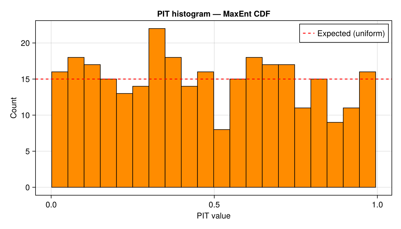

MaxEnt PIT histogram

Side-by-side comparison

fig = Figure(size = (1200, 400))

ax1 = Axis(fig[1, 1]; title = "Gregory ranks", xlabel = "Rank", ylabel = "Count")
hist!(ax1, Float64.(ranks); bins = n_bins, color = :steelblue, strokewidth = 1)
hlines!(ax1, [n_rank / n_bins]; color = :red, linestyle = :dash)

ax2 = Axis(fig[1, 2]; title = "KDE PIT", xlabel = "PIT value", ylabel = "Count")
hist!(ax2, pit_kde; bins = n_bins, color = :teal, strokewidth = 1)
hlines!(ax2, [n_rank / n_bins]; color = :red, linestyle = :dash)

ax3 = Axis(fig[1, 3]; title = "MaxEnt PIT", xlabel = "PIT value", ylabel = "Count")
hist!(ax3, pit_maxent; bins = n_bins, color = :darkorange, strokewidth = 1)
hlines!(ax3, [n_rank / n_bins]; color = :red, linestyle = :dash)

Rank histogram comparison

Mismatched observations

The observation-based interface lets us pass in observations drawn from a different distribution than the one the MLMC ensemble simulates. This is useful for diagnosing model misspecification.

Wider observations — observations from $\mathcal{N}(2,\,1^2)$ while the ensemble simulates $\mathcal{N}(2,\,0.5^2)$. Because the observations have larger variance, they fall more often in the tails, producing a U-shaped PIT histogram.

Narrower observations — observations from $\mathcal{N}(2,\,0.25^2)$ while the ensemble simulates $\mathcal{N}(2,\,0.5^2)$. The observations are concentrated near the centre, producing a peaked PIT histogram.

obs_wider   = [μ_true + 1.0  * randn() for _ in 1:n_rank]   # σ_obs = 1.0
obs_narrower = [μ_true + 0.25 * randn() for _ in 1:n_rank]   # σ_obs = 0.25

pit_wider = rank_histogram_cdf(obs_wider, levels, Function[qoi_function],
                               samples_per_level,
                               estimate_cdf_mlmc_kernel_density,
                               draw_parameters)

pit_narrower = rank_histogram_cdf(obs_narrower, levels, Function[qoi_function],
                                  samples_per_level,
                                  estimate_cdf_mlmc_kernel_density,
                                  draw_parameters)

fig = Figure(size = (1200, 400))

ax1 = Axis(fig[1, 1]; title = "Matched obs (σ = 0.5)",
           xlabel = "PIT value", ylabel = "Count")
hist!(ax1, pit_kde; bins = n_bins, color = :teal, strokewidth = 1)
hlines!(ax1, [n_rank / n_bins]; color = :red, linestyle = :dash)

ax2 = Axis(fig[1, 2]; title = "Wider obs (σ = 1.0)",
           xlabel = "PIT value", ylabel = "Count")
hist!(ax2, pit_wider; bins = n_bins, color = :coral, strokewidth = 1)
hlines!(ax2, [n_rank / n_bins]; color = :red, linestyle = :dash)

ax3 = Axis(fig[1, 3]; title = "Narrower obs (σ = 0.25)",
           xlabel = "PIT value", ylabel = "Count")
hist!(ax3, pit_narrower; bins = n_bins, color = :goldenrod, strokewidth = 1)
hlines!(ax3, [n_rank / n_bins]; color = :red, linestyle = :dash)

Mismatched rank histograms

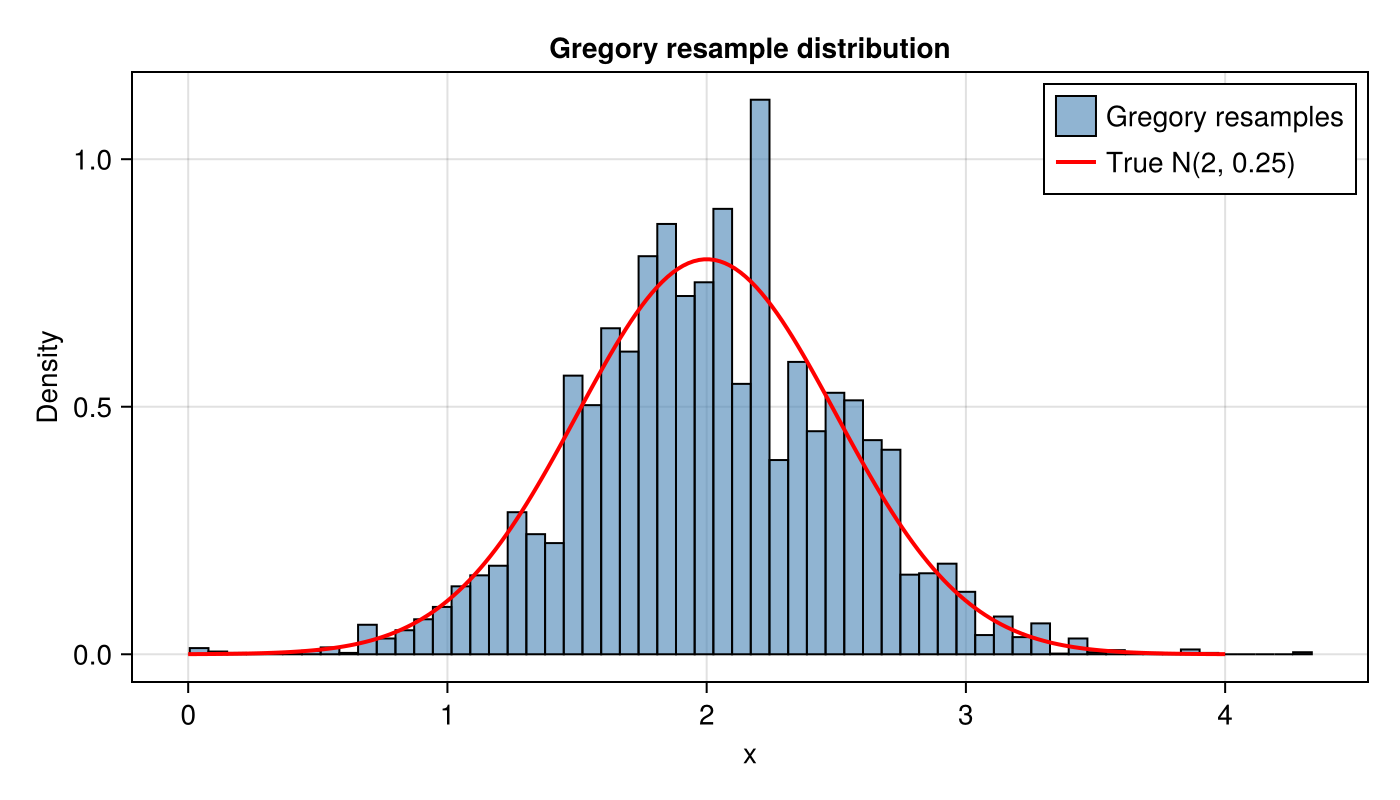
Gregory resample distribution

We can also inspect the distribution of Gregory resamples directly. Here we draw one large MLMC ensemble and resample from it:

large_samples = mlmc_sample(levels, Function[qoi_function],
                            [4000, 2000, 500], draw_parameters)
resampled = ml_gregory_resample(large_samples, 1, 10_000)

fig = Figure(size = (700, 400))
ax = Axis(fig[1, 1]; title = "Gregory resample distribution",
          xlabel = "x", ylabel = "Density")
hist!(ax, resampled; bins = 60, normalization = :pdf,
      color = (:steelblue, 0.6), strokewidth = 1, label = "Gregory resamples")

# Overlay true N(μ, σ²) density
xs = range(μ_true - 4σ_true, μ_true + 4σ_true; length = 200)
true_pdf = @. exp(-0.5 * ((xs - μ_true) / σ_true)^2) / (σ_true * sqrt(2π))
lines!(ax, xs, true_pdf; color = :red, linewidth = 2, label = "True N(2, 0.25)")
axislegend(ax; position = :rt)

Gregory resample distribution