Projectile Motion

This example demonstrates MLMC estimation applied to a projectile motion model with uncertain parameters (initial height, speed, angle, mass, drag).

Problem Setup

We define a simple projectile simulation with drag and wrap it as an MLMC hierarchy by varying the time-step resolution.

using Parameters
using Random

Random.seed!(123)

@with_kw struct Drag{RhoType, CdType, AreaType}
    ρ::RhoType = 1.225
    C_d::CdType = 0.47
    A::AreaType = 0.01
end

function (d::Drag)(v)
    return 0.5 * d.ρ * d.C_d * d.A * v^2
end

@with_kw struct ProjectileParameters{HeightType, SpeedType, AngleType, MassType, DragType}
    initial_height::HeightType
    initial_speed::SpeedType
    angle_in_degrees::AngleType
    mass::MassType
    drag::DragType
end

import Random: rand

function rand(p::ProjectileParameters)
    ProjectileParameters(
        initial_height = p.initial_height isa Real ? p.initial_height : rand(p.initial_height),
        initial_speed  = p.initial_speed  isa Real ? p.initial_speed  : rand(p.initial_speed),
        angle_in_degrees = p.angle_in_degrees isa Real ? p.angle_in_degrees : rand(p.angle_in_degrees),
        mass = p.mass isa Real ? p.mass : rand(p.mass),
        drag = Drag(
            ρ   = p.drag.ρ   isa Real ? p.drag.ρ   : rand(p.drag.ρ),
            C_d = p.drag.C_d isa Real ? p.drag.C_d : rand(p.drag.C_d),
            A   = p.drag.A   isa Real ? p.drag.A   : rand(p.drag.A),
        ),
    )
end

function projectile_motion(p::ProjectileParameters; endtime=5.0, resolution=0.01)
    g = 9.81
    θ = deg2rad(p.angle_in_degrees)
    vx, vy = p.initial_speed * cos(θ), p.initial_speed * sin(θ)
    dt = resolution
    ts = collect(0.0:dt:endtime)
    xs = zeros(length(ts))
    ys = zeros(length(ts))
    xs[1] = 0.0
    ys[1] = Float64(p.initial_height)
    last_i = 1
    for i in 2:length(ts)
        v = sqrt(vx^2 + vy^2)
        fd = p.drag(v)
        vx += (-fd * vx / v / p.mass) * dt
        vy += (-g - fd * vy / v / p.mass) * dt
        xs[i] = xs[i-1] + vx * dt
        ys[i] = ys[i-1] + vy * dt
        last_i = i
        ys[i] < 0 && break
    end
    return (x=xs[1:last_i], y=ys[1:last_i])
end

Define Uncertain Parameters

using Distributions

parameters_uncertain = ProjectileParameters(
    initial_height = Uniform(1.5, 1.7),
    initial_speed  = Uniform(8, 12),
    angle_in_degrees = Uniform(30, 60),
    mass = Uniform(0.1, 0.5),
    drag = Drag(ρ=Uniform(1.0, 1.5), C_d=Uniform(0.3, 0.6), A=Uniform(0.005, 0.015)),
)

Define MLMC Levels and QoI Functions

The levels are the same physical model run at different time-step resolutions. The QoI functions extract scalar quantities from the model output.

using MultilevelMonteCarlo

timestepsizes = 2.0 .^ (-2:-1:-6)

levels = Function[
    let dt = dt
        params -> projectile_motion(params; endtime=5.0, resolution=dt)
    end
    for dt in timestepsizes
]

qoi_distance(output)   = maximum(output.x)
qoi_max_height(output) = maximum(output.y)
qoi_functions = Function[qoi_distance, qoi_max_height]

Variance Estimation and Optimal Allocation

samples_per_level = fill(1024, length(timestepsizes))

variances_corrections, variances = variance_per_level(
    levels, qoi_functions, samples_per_level,
    () -> rand(parameters_uncertain),
)

println("Variance of corrections: ", round.(variances_corrections, sigdigits=3))
println("Variance per level:      ", round.(variances, sigdigits=3))

Variance of corrections: [96.2, 27.2, 6.44, 1.75]
Variance per level:      [1780.0, 1970.0, 2210.0, 2100.0, 2200.0]

Compute the optimal sample allocation for a given tolerance:

tolerance = 0.1
cost_per_level = timestepsizes .^ (-1)

samples_optimal = optimal_samples_per_level(
    variances_corrections, variances, cost_per_level, tolerance,
)
println("Optimal samples per level: ", samples_optimal)

Optimal samples per level: [666200, 109543, 41217, 14173, 5216]

MLMC Estimation (Scalar QoIs)

result = mlmc_estimate(
    levels, qoi_functions, samples_per_level,
    () -> rand(parameters_uncertain),
)
println("MLMC estimates: distance = ", round(result[1], digits=3),
        ", max height = ", round(result[2], digits=3))

MLMC estimates: distance = 10.218, max height = 3.986

Mean Trajectory: MLMC vs Monte Carlo

To compute the mean trajectory $E[y(x)]$, we define a vector-valued QoI that interpolates each simulated trajectory onto a common horizontal grid.

# Fixed horizontal grid for trajectory interpolation
const x_grid = collect(range(0, 10, length=100))

function interp_trajectory(x_traj, y_traj, xg)
    n = length(x_traj)
    result = zeros(length(xg))
    for (i, xv) in enumerate(xg)
        if xv <= x_traj[1]
            result[i] = y_traj[1]
        elseif xv >= x_traj[end]
            result[i] = 0.0
        else
            idx = searchsortedlast(x_traj, xv)
            frac = (xv - x_traj[idx]) / (x_traj[idx+1] - x_traj[idx])
            result[i] = (1 - frac) * y_traj[idx] + frac * y_traj[idx+1]
        end
        result[i] = max(0.0, result[i])
    end
    return result
end

qoi_trajectory(output) = interp_trajectory(output.x, output.y, x_grid)

# MLMC mean trajectory
mlmc_traj = mlmc_estimate_vector_qoi(
    levels, qoi_trajectory, samples_per_level,
    () -> rand(parameters_uncertain),
)

# MC mean trajectory (same total work, finest level only)
mc_traj = evaluate_monte_carlo_vector_qoi(
    2000,
    () -> rand(parameters_uncertain),
    levels[end],
    qoi_trajectory,
)

using CairoMakie

fig = Figure(size=(700, 400))
ax = Axis(fig[1, 1]; xlabel="Horizontal distance (m)", ylabel="Height (m)",
          title="Mean Trajectory: MLMC vs Monte Carlo")
lines!(ax, x_grid, mlmc_traj; label="MLMC mean", color=:blue, linewidth=2)
lines!(ax, x_grid, mc_traj; label="MC mean (finest level)", color=:red,
       linewidth=2, linestyle=:dash)
axislegend(ax; position=:rt)
fig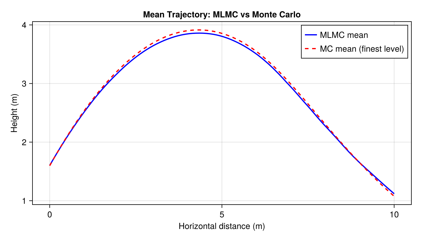

Adaptive MLMC

The adaptive variant iteratively refines sample counts to meet the target tolerance:

adaptive_result, adaptive_counts = mlmc_estimate_adaptive(
    levels, qoi_functions,
    () -> rand(parameters_uncertain),
    cost_per_level, tolerance;
    initial_samples = 100,
)
println("Adaptive MLMC: distance = ", round(adaptive_result[1], digits=3),
        ", max height = ", round(adaptive_result[2], digits=3))
println("Final sample counts: ", adaptive_counts)

Adaptive MLMC: distance = 10.327, max height = 4.002
Final sample counts: [678022, 110030, 44091, 15250, 5348]