Projectile in Wind

This example demonstrates 3-D projectile motion under an uncertain wind field generated with GaussianRandomFields.jl. The Euler integration timestep determines the MLMC level, and the QoIs are the landing coordinates $(x_{\mathrm{land}},\, y_{\mathrm{land}})$.

Model

A projectile is launched from the origin with uncertain initial velocity $\mathbf{v}_0 = (v_{x0},\, v_{y0},\, v_{z0})$. During flight it experiences gravity and a random wind acceleration that varies with time. The wind components $w_x(t)$ and $w_y(t)$ are independent samples from a 1-D Gaussian random field with exponential covariance on the time axis.

The equations of motion are

\[\ddot{x} = w_x(t),\qquad \ddot{y} = w_y(t),\qquad \ddot{z} = -g.\]

The projectile lands when $z$ crosses zero from above.

Setup

using MultilevelMonteCarlo
using GaussianRandomFields
using CairoMakie
using Statistics
using Random
Random.seed!(123)

const g_acc = 9.81
const T_max = 6.0   # generous upper bound on flight time

# --- Wind field: 1-D GRF along the time axis ---
n_wind  = 301
t_wind  = range(0, T_max; length = n_wind)
cov_fn  = CovarianceFunction(1, Exponential(1.5))        # length-scale 1.5 s
grf_wind = GaussianRandomField(cov_fn, Cholesky(), t_wind)

# Linear interpolation helper
function _wind_at(vals, t)
    t <= t_wind[1]   && return vals[1]
    t >= t_wind[end]  && return vals[end]
    idx = searchsortedlast(t_wind, t)
    idx = clamp(idx, 1, length(t_wind) - 1)
    α = (t - t_wind[idx]) / (t_wind[idx+1] - t_wind[idx])
    return (1 - α) * vals[idx] + α * vals[idx+1]
end

# Uncertain parameters: initial velocity + wind realisation
function draw_params()
    vx0 = 20.0 + 1.0 * randn()
    vy0 =  0.0 + 1.0 * randn()
    vz0 = 20.0 + 1.0 * randn()
    wx  = 2.0 .* GaussianRandomFields.sample(grf_wind)
    wy  = 2.0 .* GaussianRandomFields.sample(grf_wind)
    return (vx0, vy0, vz0, wx, wy)
end

Level functions

Each level uses a different Euler-integration timestep. Finer levels yield more accurate landing positions.

function make_level(dt)
    function simulate(params)
        vx0, vy0, vz0, wx, wy = params
        x, y, z     = 0.0, 0.0, 0.0
        vx, vy, vz  = vx0, vy0, vz0
        t = 0.0

        x_prev, y_prev, z_prev = x, y, z
        while true
            ax = _wind_at(wx, t)
            ay = _wind_at(wy, t)

            x_prev, y_prev, z_prev = x, y, z
            vx += ax * dt;  vy += ay * dt;  vz -= g_acc * dt
            x  += vx * dt;  y  += vy * dt;  z  += vz * dt
            t  += dt

            if z <= 0.0 || t >= T_max
                # Linearly interpolate to z = 0 crossing
                if z_prev > 0.0 && z < 0.0
                    α = z_prev / (z_prev - z)
                    x = x_prev + α * (x - x_prev)
                    y = y_prev + α * (y - y_prev)
                end
                break
            end
        end
        return [x, y]
    end
    return simulate
end

levels = Function[make_level(0.1), make_level(0.02), make_level(0.004)]
qoi_functions = Function[r -> r[1], r -> r[2]]

Sample trajectories

fig = Figure(size = (900, 600))
ax = Axis3(fig[1, 1]; title = "Sample 3-D trajectories",
           xlabel = "x [m]", ylabel = "y [m]", zlabel = "z [m]")

for _ in 1:10
    params = draw_params()
    vx0, vy0, vz0, wx, wy = params
    traj_x, traj_y, traj_z = Float64[], Float64[], Float64[]
    x, y, z = 0.0, 0.0, 0.0
    vx, vy, vz = vx0, vy0, vz0
    dt = 0.004;  t = 0.0
    push!(traj_x, x); push!(traj_y, y); push!(traj_z, z)
    while z >= 0.0 && t < T_max
        vx += _wind_at(wx, t) * dt
        vy += _wind_at(wy, t) * dt
        vz -= g_acc * dt
        x  += vx * dt;  y += vy * dt;  z += vz * dt
        t  += dt
        push!(traj_x, x); push!(traj_y, y); push!(traj_z, max(z, 0.0))
    end
    lines!(ax, traj_x, traj_y, traj_z; linewidth = 1.5)
end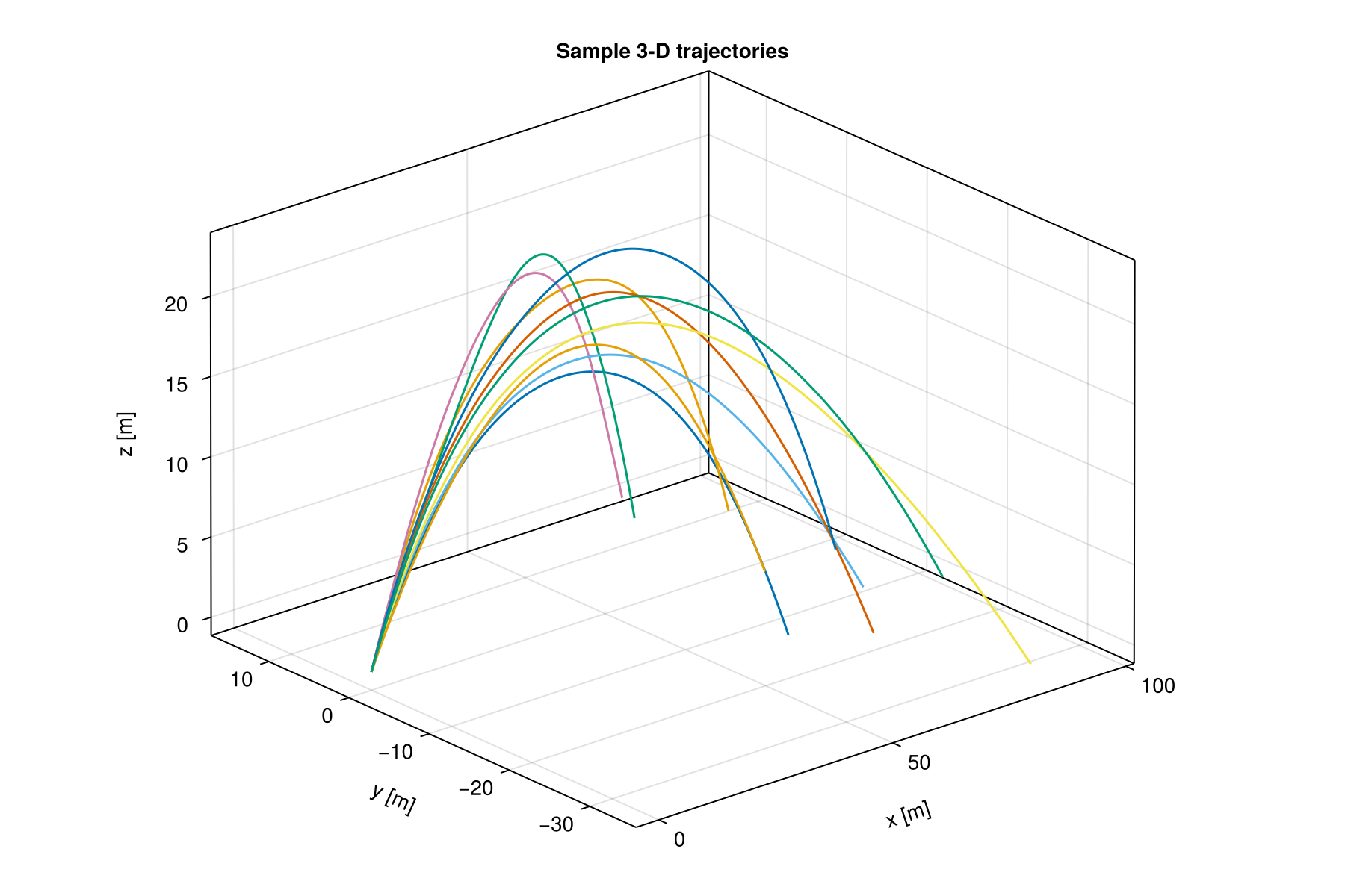

MLMC samples and landing scatter

samples_per_level = [1500, 500, 150]
samples = mlmc_sample(levels, qoi_functions, samples_per_level, draw_params)

ens = ml_bootstrap_resample_multivariate(samples, [1, 2], 5000)

fig = Figure(size = (700, 500))
ax = Axis(fig[1, 1]; title = "Bootstrap resamples — landing position",
          xlabel = "x [m]", ylabel = "y [m]")
scatter!(ax, ens[1, :], ens[2, :]; markersize = 3,
         color = (:steelblue, 0.3))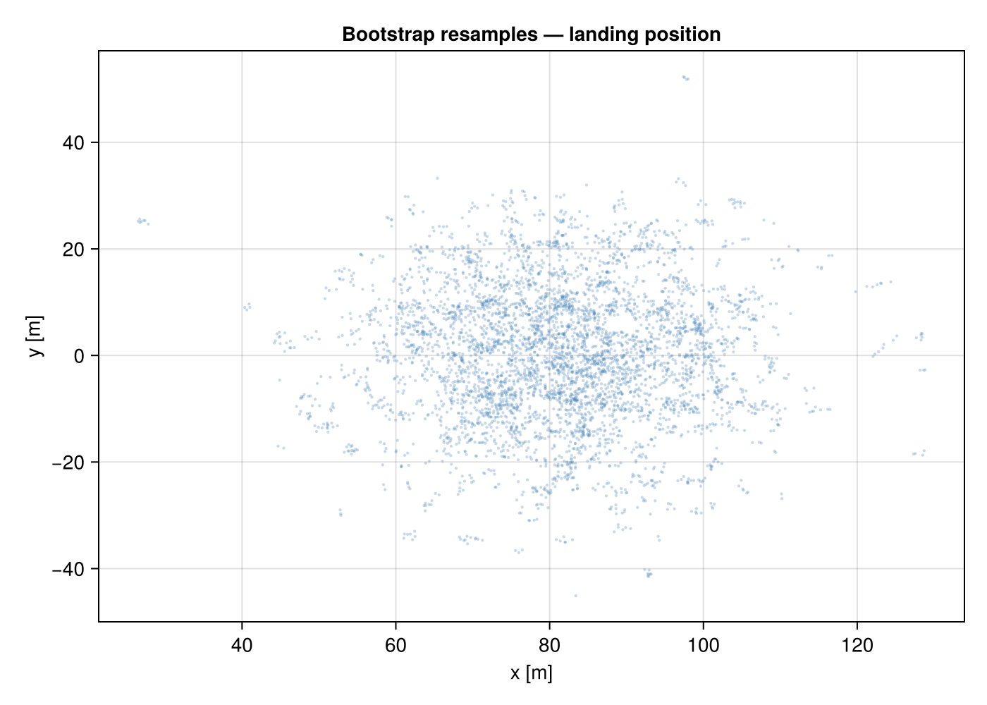

2-D CDF of landing position

F̂_kde = estimate_cdf_mlmc_kernel_density_2d(samples, (1, 2))

x_grid = range(quantile(ens[1, :], 0.01), quantile(ens[1, :], 0.99); length = 50)
y_grid = range(quantile(ens[2, :], 0.01), quantile(ens[2, :], 0.99); length = 50)
cdf_vals = [F̂_kde(x1, x2) for x2 in y_grid, x1 in x_grid]

fig = Figure(size = (700, 500))
ax = Axis(fig[1, 1]; title = "MLMC KDE CDF — landing position",
          xlabel = "x [m]", ylabel = "y [m]")
co = contourf!(ax, collect(x_grid), collect(y_grid), cdf_vals;
               levels = 0.0:0.1:1.0, colormap = :viridis)
Colorbar(fig[1, 2], co; label = "F̂(x, y)")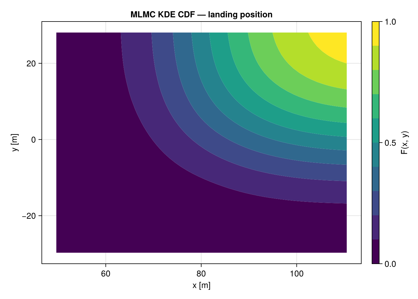

Multivariate rank histogram

We use the default KDE-based CDF method inside multivariate_rank_histogram to assess the joint calibration of the MLMC estimate for the 2-D landing position.

n_rank = 120
n_resamples = 250

pit_wind = multivariate_rank_histogram(
    levels, qoi_functions, draw_params,
    n_rank, samples_per_level;
    number_of_resamples = n_resamples,
)

n_bins = 12
fig = Figure(size = (700, 400))
ax = Axis(fig[1, 1]; title = "MRH — landing position",
          xlabel = "PIT value", ylabel = "Count")
hist!(ax, pit_wind; bins = n_bins, color = :mediumpurple, strokewidth = 1)
hlines!(ax, [n_rank / n_bins]; color = :red, linestyle = :dash,
        label = "Expected (uniform)")
axislegend(ax; position = :rt)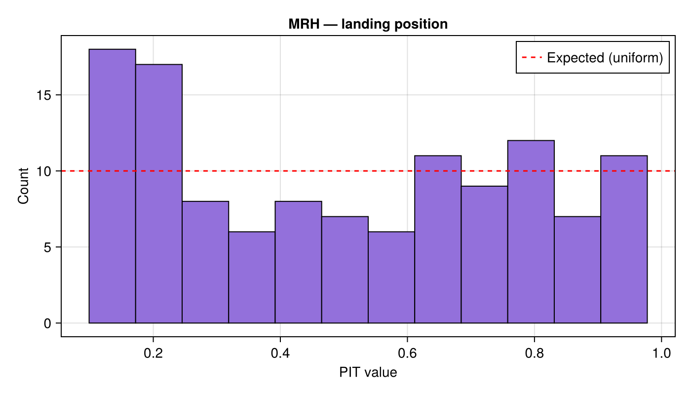

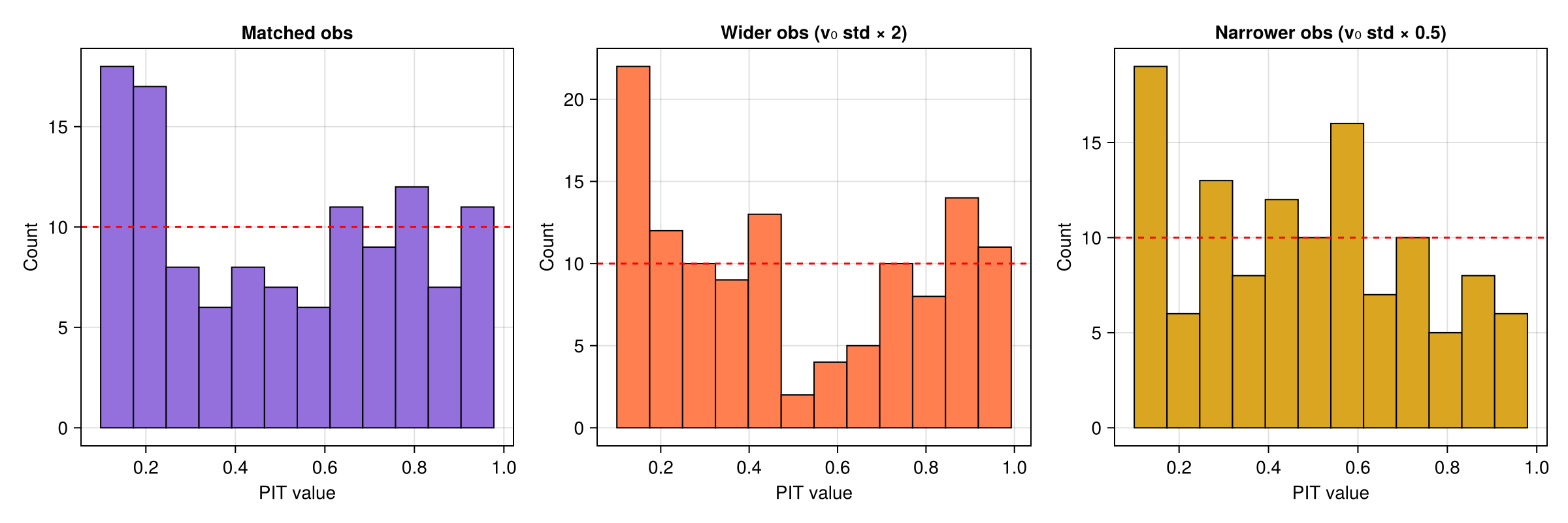
Mismatched observations

We can test robustness by passing in observations with perturbed initial velocity distributions.

Wider observations — initial velocity std doubled ($2.0$ instead of $1.0$), producing landings that spread beyond the ensemble.

Narrower observations — initial velocity std halved ($0.5$ instead of $1.0$), producing landings concentrated near the mean.

function draw_params_wider()
    vx0 = 20.0 + 2.0 * randn()
    vy0 =  0.0 + 2.0 * randn()
    vz0 = 20.0 + 2.0 * randn()
    wx  = 2.0 .* GaussianRandomFields.sample(grf_wind)
    wy  = 2.0 .* GaussianRandomFields.sample(grf_wind)
    return (vx0, vy0, vz0, wx, wy)
end

function draw_params_narrower()
    vx0 = 20.0 + 0.5 * randn()
    vy0 =  0.0 + 0.5 * randn()
    vz0 = 20.0 + 0.5 * randn()
    wx  = 2.0 .* GaussianRandomFields.sample(grf_wind)
    wy  = 2.0 .* GaussianRandomFields.sample(grf_wind)
    return (vx0, vy0, vz0, wx, wy)
end

# Generate observations from each distribution
obs_wider = hcat([let p = draw_params_wider(); r = levels[end](p); [qoi_functions[1](r), qoi_functions[2](r)] end for _ in 1:n_rank]...)
obs_narrower = hcat([let p = draw_params_narrower(); r = levels[end](p); [qoi_functions[1](r), qoi_functions[2](r)] end for _ in 1:n_rank]...)

pit_wider = multivariate_rank_histogram(obs_wider, levels, qoi_functions,
                                        samples_per_level, draw_params;
                                        number_of_resamples = n_resamples)

pit_narrower = multivariate_rank_histogram(obs_narrower, levels, qoi_functions,
                                           samples_per_level, draw_params;
                                           number_of_resamples = n_resamples)

fig = Figure(size = (1200, 400))

ax1 = Axis(fig[1, 1]; title = "Matched obs",
           xlabel = "PIT value", ylabel = "Count")
hist!(ax1, pit_wind; bins = n_bins, color = :mediumpurple, strokewidth = 1)
hlines!(ax1, [n_rank / n_bins]; color = :red, linestyle = :dash)

ax2 = Axis(fig[1, 2]; title = "Wider obs (v₀ std × 2)",
           xlabel = "PIT value", ylabel = "Count")
hist!(ax2, pit_wider; bins = n_bins, color = :coral, strokewidth = 1)
hlines!(ax2, [n_rank / n_bins]; color = :red, linestyle = :dash)

ax3 = Axis(fig[1, 3]; title = "Narrower obs (v₀ std × 0.5)",
           xlabel = "PIT value", ylabel = "Count")
hist!(ax3, pit_narrower; bins = n_bins, color = :goldenrod, strokewidth = 1)
hlines!(ax3, [n_rank / n_bins]; color = :red, linestyle = :dash)