Urban landscape

This example demonstrates the application of static and dynamic functionality in SWIM in an urban setting using real data. The example is from the 'Kuba' area in central Oslo. The topography with some steep hills and a high degree of impermeable surfaces makes the area sensitive to intense rainfall events.

Loading the necessary packages

using SurfaceWaterIntegratedModeling
import CairoMakie, Images # for visualization and loading of textures
import ColorSchemes
using Pkg.Artifacts
import ArchGDAL # for loading of topographical grids from files in geotiff format

Prepare data

The package with SWIM testdata is provided as a Julia artifact, which can be accessed using the function datapath_testdata. We subsequently load a digital surface model (including buildings and vegetation) and a digtial terrain model (without buildings or vegetation) of the area of study ^[1]. The data is converted into simple Julia arrays with height values stored as Float64.

kuba_datapath = joinpath(datapath_testdata(), "data", "kuba")
geoarray_dsm = ArchGDAL.readraster(joinpath(kuba_datapath, "dom1", "data", "dom1.tif"))
geoarray_dtm = ArchGDAL.readraster(joinpath(kuba_datapath, "dtm1", "data", "dtm1.tif"))

grid_dtm = permutedims(geoarray_dtm[:,:,1]) .|> Float64
grid_dsm = permutedims(geoarray_dsm[:,:,1]) .|> Float64
typeof(grid_dtm), size(grid_dtm)

(Matrix{Float64}, (649, 745))

In addition to the elevation data, we also load a set of textures and masks that can be used to visualize the model, as well as indicate the locations of buildings, permeable areas, rivers and sinks (e.g. manholes).

mapimg = Images.load(joinpath(kuba_datapath, "textures", "kuba.png"))
photoimg = Images.load(joinpath(kuba_datapath, "textures", "kuba_photo.png"))

building_mask = Images.load(joinpath(kuba_datapath, "textures", "building_mask.png"))
pavement_mask = Images.load(joinpath(kuba_datapath, "textures", "pavement_mask.png"))
river_mask = Images.load(joinpath(kuba_datapath, "textures", "river_mask.png"))
permeable_mask = Images.load(joinpath(kuba_datapath, "textures", "permeable_mask.png"))
sink_mask = Images.load(joinpath(kuba_datapath, "textures", "sink_mask.png"))
typeof(sink_mask), size(sink_mask)

(Matrix{ColorTypes.Gray{FixedPointNumbers.N0f8}}, (1333, 1522))

The textures are not all of the same resolution. We resize them all to equal resolution; twice the topographical grid resolution in both directions.

mapimg = Images.imresize(mapimg, size(grid_dtm) .* 2)
photoimg = Images.imresize(photoimg, size(mapimg))

building_mask = Images.imresize(building_mask, size(mapimg))
pavement_mask = Images.imresize(pavement_mask, size(mapimg))
river_mask = Images.imresize(river_mask, size(mapimg))
permeable_mask = Images.imresize(permeable_mask, size(mapimg))
sink_mask = Images.imresize(sink_mask, size(mapimg))
size(sink_mask)

(1298, 1490)

We can visualize the model surfaces with the textures to see how the area looks. Here, we show the terrain model with the map texture and the surface model with the aerial photo texture.

sfmap, figmap, scmap = plotgrid(grid_dtm, texture=mapimg)
sfpho, figpho, scpho = plotgrid(grid_dsm, texture=photoimg)

(MakieCore.Mesh{Tuple{GeometryBasics.Mesh{3, Float32, GeometryBasics.TriangleP{3, Float32, GeometryBasics.PointMeta{3, Float32, GeometryBasics.Point{3, Float32}, (:uv, :normals), Tuple{GeometryBasics.Vec{2, Float32}, GeometryBasics.Point{3, Float32}}}}, GeometryBasics.FaceView{GeometryBasics.TriangleP{3, Float32, GeometryBasics.PointMeta{3, Float32, GeometryBasics.Point{3, Float32}, (:uv, :normals), Tuple{GeometryBasics.Vec{2, Float32}, GeometryBasics.Point{3, Float32}}}}, GeometryBasics.PointMeta{3, Float32, GeometryBasics.Point{3, Float32}, (:uv, :normals), Tuple{GeometryBasics.Vec{2, Float32}, GeometryBasics.Point{3, Float32}}}, GeometryBasics.NgonFace{3, GeometryBasics.OffsetInteger{-1, UInt32}}, StructArrays.StructVector{GeometryBasics.PointMeta{3, Float32, GeometryBasics.Point{3, Float32}, (:uv, :normals), Tuple{GeometryBasics.Vec{2, Float32}, GeometryBasics.Point{3, Float32}}}, @NamedTuple{position::Vector{GeometryBasics.Point{3, Float32}}, uv::Vector{GeometryBasics.Vec{2, Float32}}, normals::Vector{GeometryBasics.Point{3, Float32}}}, Int64}, Vector{GeometryBasics.NgonFace{3, GeometryBasics.OffsetInteger{-1, UInt32}}}}}}}, Scene (800px, 600px):
  0 Plots
  1 Child Scene:
    └ Scene (768px, 568px), Scene (768px, 568px):
  2 Plots:
    ├ MakieCore.Combined{Makie.axis3d, Tuple{Tuple{Tuple{Float32, Float32}, Tuple{Float32, Float32}, Tuple{Float32, Float32}}}}
    └ MakieCore.Mesh{Tuple{GeometryBasics.Mesh{3, Float32, GeometryBasics.TriangleP{3, Float32, GeometryBasics.PointMeta{3, Float32, GeometryBasics.Point{3, Float32}, (:uv, :normals), Tuple{GeometryBasics.Vec{2, Float32}, GeometryBasics.Point{3, Float32}}}}, GeometryBasics.FaceView{GeometryBasics.TriangleP{3, Float32, GeometryBasics.PointMeta{3, Float32, GeometryBasics.Point{3, Float32}, (:uv, :normals), Tuple{GeometryBasics.Vec{2, Float32}, GeometryBasics.Point{3, Float32}}}}, GeometryBasics.PointMeta{3, Float32, GeometryBasics.Point{3, Float32}, (:uv, :normals), Tuple{GeometryBasics.Vec{2, Float32}, GeometryBasics.Point{3, Float32}}}, GeometryBasics.NgonFace{3, GeometryBasics.OffsetInteger{-1, UInt32}}, StructArrays.StructVector{GeometryBasics.PointMeta{3, Float32, GeometryBasics.Point{3, Float32}, (:uv, :normals), Tuple{GeometryBasics.Vec{2, Float32}, GeometryBasics.Point{3, Float32}}}, @NamedTuple{position::Vector{GeometryBasics.Point{3, Float32}}, uv::Vector{GeometryBasics.Vec{2, Float32}}, normals::Vector{GeometryBasics.Point{3, Float32}}}, Int64}, Vector{GeometryBasics.NgonFace{3, GeometryBasics.OffsetInteger{-1, UInt32}}}}}}}
  0 Child Scenes)

The plotgrid function creates a 3D scene. If GLMakie is used, the scene is displayed in a graphical window that can be navigated using the keyboard and mouse. The viewpoint of the scene can also be changed programatically using set_camerapos. We predefine a couple of viewpoints on the form (camera position, target, zoomlevel):

view1 = (CairoMakie.Vec(1223, 587, 1056), CairoMakie.Vec(391, 327, 13.8), 0.66)
view2 = (CairoMakie.Vec(1223, 587, 1056), CairoMakie.Vec(391, 327, 13.8), 0.30);

Here is a snapshot for the terrain model:

figmap
set_camerapos(figmap, scmap, view1...)

And a snapshot of the surface model:

figpho
set_camerapos(figpho, scpho, view1...)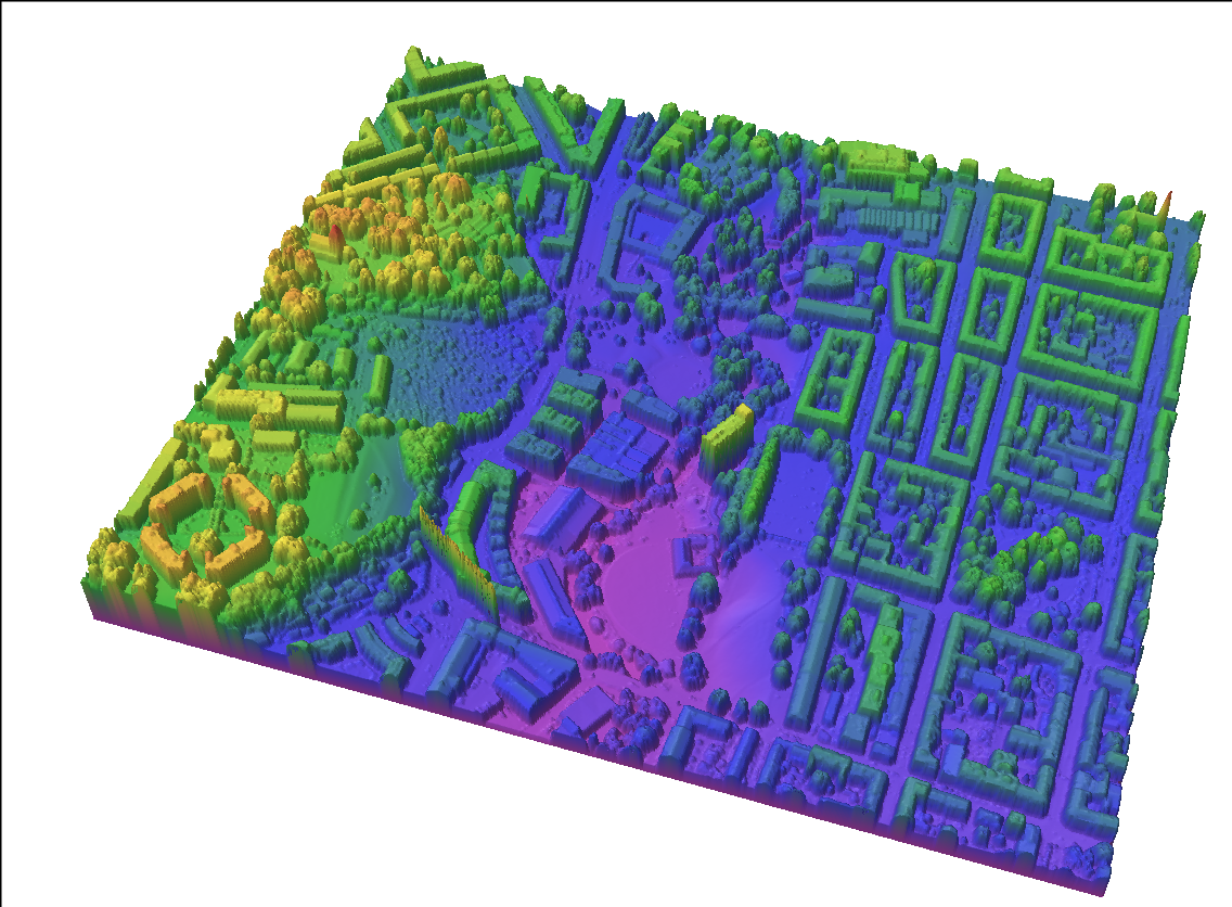

Here is a visualization of the different masks loaded:

fig = CairoMakie.Figure()
maskarray = [building_mask, pavement_mask, river_mask, permeable_mask, sink_mask]
masktitles= ["Building mask", "Pavement mask", "River mask", "Permeable mask", "Sink mask"]
fig_axes = []
for i = 1:5
    push!(fig_axes, CairoMakie.Axis(fig[Int(ceil(i/3)), mod(i-1, 3)+1]))
    CairoMakie.image!(fig_axes[end], rotr90(maskarray[i]))
    fig_axes[end].title = masktitles[i]
end
fig_yres = Int(ceil(size(building_mask, 2) / 3))
CairoMakie.resize!(fig.scene, fig_yres * 3, fig_yres * 2)
fig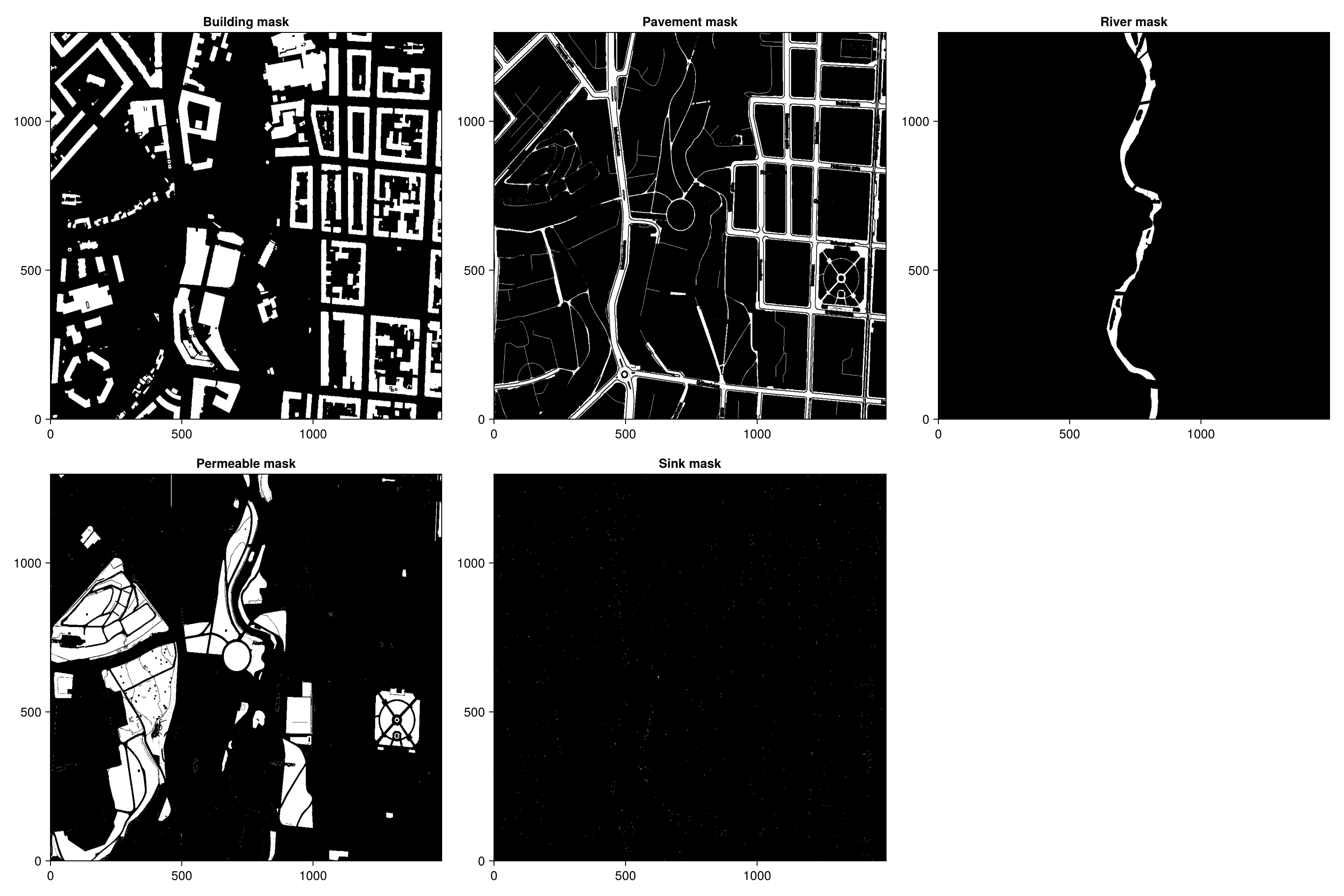

Prepare and run the static analysis

In this step, we run a static analysis on the terrain, to determine the following information:

The flow pattern of water on the terrain, i.e. how water moves from one grid-cell to the next, assuming infinitesimal, gravity-driven flow.
Identify accumulation regions (lakes), and two related tree-like hierarchies:
- How separate lakes merge as they grow (subtraps -> supertraps)
- How lakes, once full, pour into lakes further downstream (upstream traps -> downstream traps)

We run the analysis twice. In the first run we only consider the impact of buildings, in the second we also include sinks in the analysis.

The spillanalysis function requires that overlay masks indicating buildings or sinks have the same resolution as the topographical grid. We therefore resize building- and sink masks below. Note that in the input data, sinks are often represented as a single pixel, so they risk disappearing in the downsampling process. To prevent this, we downsample the grids as full grayscale images, and then quantify to a logical mask where all completely black pixels are set to false and all other pixels set to true.

Downsampling the building and sink masks

(The river is also treated as a sink here).

bmask = Images.imresize(building_mask, size(grid_dtm))
bmask[bmask .!= Images.Gray{Images.N0f8}(0.0)] .= Images.Gray{Images.N0f8}(1.0)
bmask = Matrix{Bool}(bmask .== Images.Gray{Images.N0f8}(1.0))

smask = Images.imresize(sink_mask + river_mask, size(grid_dtm))
smask[smask .!= Images.Gray{Images.N0f8}(0.0)] .= Images.Gray{Images.N0f8}(1.0)
smask = Matrix{Bool}(smask .== Images.Gray{Images.N0f8}(1.0));

Run the two spill analyses

tstruct_nosinks = spillanalysis(grid_dtm, building_mask=bmask)
tstruct_sinks = spillanalysis(grid_dtm, building_mask=bmask, sinks=smask);

# Visualize the result of the static analyses

TrapStructure{Float64}([0.0 39.688663482666016 … 30.804061889648438 0.0; 0.0 39.59254837036133 … 30.780582427978516 0.0; … ; 0.0 37.69725799560547 … 13.538226127624512 0.0; 0.0 0.0 … 0.0 0.0], Int8[-2 -2 … 3 3; -2 -2 … 3 3; … ; 2 1 … -2 -2; -1 1 … -2 -2], [0 0 … -13773 -13773; 0 0 … -13774 -13774; … ; -539 -542 … 0 0; -540 -542 … 0 0], Spillpoint[Spillpoint(128, 33789, 34438, 34.84395217895508), Spillpoint(-35, 1354, 704, 37.43061828613281), Spillpoint(120, 24715, 25363, 35.30595016479492), Spillpoint(18, 3344, 3992, 37.343772888183594), Spillpoint(34, 4651, 5299, 37.38553237915039), Spillpoint(19, 2731, 3380, 38.173336029052734), Spillpoint(8, 1462, 2112, 40.283992767333984), Spillpoint(88, 18315, 18963, 38.242835998535156), Spillpoint(-553, 3496, 4144, 49.097076416015625), Spillpoint(53, 7522, 8171, 40.81281280517578)  …  Spillpoint(954, 181846, 181198, 16.580142974853516), Spillpoint(-12442, 313714, 313065, 20.968334197998047), Spillpoint(1384, 237191, 237839, 15.311931610107422), Spillpoint(889, 165323, 165322, 17.637786865234375), Spillpoint(966, 174115, 174114, 16.474254608154297), Spillpoint(898, 164682, 164033, 17.924983978271484), Spillpoint(-1654, 183226, 183874, 16.475128173828125), Spillpoint(863, 163383, 162735, 17.92721176147461), Spillpoint(912, 165343, 165344, 17.930648803710938), Spillpoint(-1544, 165346, 165995, 17.942995071411133)], [0.0053863525390625, 0.5009384155273438, 0.003143310546875, 0.016918182373046875, 0.43630218505859375, 0.06953811645507812, 0.11246871948242188, 0.006229400634765625, 0.026638031005859375, 0.002010345458984375  …  9.070137023925781, 599.0291118621826, 57.357826232910156, 239.02290153503418, 14.313800811767578, 383.9362211227417, 14.577449798583984, 384.67076778411865, 475.0479688644409, 481.94111347198486], [0.0, 0.0, 0.0, 0.0, 0.0, 0.0, 0.0, 0.0, 0.0, 0.0  …  3.739492416381836, 523.9987449645996, 38.22144031524658, 128.1084747314453, 12.389406204223633, 298.0799169540405, 14.315185546875, 383.93859577178955, 473.2034025192261, 475.0544557571411], [[33789], [1354, 2003, 2004, 2652, 2653, 3302, 3951], [24715], [2695, 3344, 3345], [2054, 2703, 2704, 2705, 3352, 3353, 3354, 3355, 4001, 4002, 4003, 4004, 4651, 4652, 4653, 4654], [1432, 2082, 2731], [1461, 1462], [17666, 17667, 18315], [2847, 3496, 3497], [7522]  …  [170807, 170808, 170809, 171453, 171454, 171455, 171456, 171457, 171458, 172102  …  192878, 192879, 193528, 194177, 194826, 194827, 195475, 195476, 195477, 196125], [303359, 303360, 303361, 303362, 303363, 303364, 303997, 303998, 303999, 304000  …  316310, 316311, 316948, 316949, 316950, 316951, 316952, 316960, 317600, 317601], [217724, 217725, 217726, 217727, 218371, 218372, 218373, 218374, 218375, 218376  …  241744, 241745, 242387, 242388, 242389, 242390, 242391, 242392, 243037, 243038], [165323, 165973, 165974, 165975, 165976, 165977, 165978, 165979, 165980, 165983  …  184206, 184207, 184854, 184855, 184856, 184857, 185505, 185506, 185507, 186154], [174115, 174119, 174765, 174767, 174768, 174769, 174770, 175412, 175413, 175414  …  186467, 186468, 187116, 187117, 187765, 187766, 188414, 188415, 189063, 189064], [163368, 164015, 164016, 164017, 164018, 164663, 164664, 164665, 164666, 164667  …  184206, 184207, 184854, 184855, 184856, 184857, 185505, 185506, 185507, 186154], [174114, 174115, 174119, 174765, 174767, 174768, 174769, 174770, 175412, 175413  …  186468, 187116, 187117, 187765, 187766, 188414, 188415, 189063, 189064, 189712], [163368, 163383, 164015, 164016, 164017, 164018, 164033, 164663, 164664, 164665  …  184206, 184207, 184854, 184855, 184856, 184857, 185505, 185506, 185507, 186154], [160128, 160129, 160130, 160131, 160132, 160133, 160134, 160135, 160136, 160137  …  184206, 184207, 184854, 184855, 184856, 184857, 185505, 185506, 185507, 186154], [160128, 160129, 160130, 160131, 160132, 160133, 160134, 160135, 160136, 160137  …  184206, 184207, 184854, 184855, 184856, 184857, 185505, 185506, 185507, 186154]], [[1], [2], [3], [4], [5], [6], [7], [8], [9], [10]  …  [1135, 1176, 944, 1134, 1112, 1054, 1080, 1053, 1027, 1032, 1004, 945, 943], [1767, 1748, 1710, 1717, 1714, 1696, 1689, 1699, 1697, 1705, 1698, 1709], [1326, 1371, 1378, 1387, 1388, 1392, 1342, 1367, 1336, 1270, 1319, 1412, 1362], [909, 927, 935, 963, 998, 1011, 1050, 1059, 1085, 1036  …  1030, 1022, 1031, 918, 910, 911, 914, 919, 913, 904], [1057, 1114, 986, 1090, 1043, 1012, 1006, 959, 1005, 974, 1038, 1056, 973, 1013, 960], [888, 889, 909, 927, 935, 963, 998, 1011, 1050, 1059  …  1030, 1022, 1031, 918, 910, 911, 914, 919, 913, 904], [1057, 1114, 986, 1090, 1043, 1012, 1006, 959, 1005, 974, 1038, 1056, 973, 1013, 960, 966], [888, 889, 909, 927, 935, 963, 998, 1011, 1050, 1059  …  1022, 1031, 918, 910, 911, 914, 919, 913, 904, 898], [888, 889, 909, 927, 935, 963, 998, 1011, 1050, 1059  …  891, 917, 863, 867, 868, 860, 884, 890, 883, 916], [912, 888, 889, 909, 927, 935, 963, 998, 1011, 1050  …  891, 917, 863, 867, 868, 860, 884, 890, 883, 916]], [[1], [2], [3], [4], [5], [6, 3198], [7], [8], [9], [10]  …  [3187], [3188, 3694], [3189], [3190], [3191], [3192], [3193], [3194], [3195, 3574], [3196, 3574]], Graphs.SimpleGraphs.SimpleDiGraph{Int64}(1524, [Int64[], Int64[], Int64[], Int64[], Int64[], [3198], Int64[], Int64[], Int64[], Int64[]  …  Int64[], Int64[], Int64[], [3954], [3955], [3956], Int64[], [3957], [3958], Int64[]], [Int64[], Int64[], Int64[], Int64[], Int64[], Int64[], Int64[], Int64[], Int64[], Int64[]  …  [3335, 3943], [1767, 3936], [1326, 3940], [904, 3948], [960, 3945], [3300, 3952], [966, 3953], [898, 3954], [3903, 3956], [912, 3957]]), Bool[1 1 … 0 0; 1 1 … 0 0; … ; 0 0 … 1 1; 0 0 … 1 1], [(376, 2), (319, 3), (136, 4), (137, 4), (497, 4), (136, 5), (137, 5), (329, 6), (330, 6), (70, 9)  …  (599, 741), (600, 741), (599, 742), (600, 742), (117, 743), (118, 743), (620, 744), (31, 745), (32, 745), (620, 745)])

To visualize the result, we will map the identified lakes and their connections on top of the topography surface.

First, we need to define the colors used for indicating buildings and lakes. We then generate a grid indicating the presence of buildings, traps or rivers, and upsample it to match the resolution of the map/photo textures.

white_color = eltype(mapimg)(1.0, 1.0, 1.0)
blue_color = eltype(mapimg)(0.0, 0.0, 1.0)
red_color = eltype(mapimg)(1.0, 0.0, 0.0)
green_color = eltype(mapimg)(0.0, 1.0, 0.0)
black_color = eltype(mapimg)(0.0, 0.0, 0.0)
beige_color = Images.RGBA{Images.N0f8}(0.933, 0.867, 0.510); # used to indicate dry parts of lakes

tex_nosinks = show_region_selection(tstruct_nosinks, trap_color=2, river_color = 3)
tex_sinks = show_region_selection(tstruct_sinks, trap_color=2, river_color = 3)

doublesize = tex -> tex[repeat(1:size(tex, 1), 1, 2)'[:],
                        repeat(1:size(tex, 2), 1, 2)'[:]] # upsampling function
tex_nosinks = doublesize(tex_nosinks)
tex_sinks = doublesize(tex_sinks);

Traps and buildings are then written onto a copy of the textures.

overlay = copy(Images.imresize(mapimg, size(grid_dtm) .* 2))
overlay_nosinks = copy(overlay)
overlay_nosinks[building_mask .== Images.GrayA{Images.N0f8}(1.0, 1.0)] .= white_color
overlay_nosinks[tex_nosinks .== 2] .= blue_color
overlay_nosinks[tex_nosinks .== 3] .= blue_color
overlay_nosinks[river_mask .> Images.Gray{Images.N0f8}(0.0)] .= blue_color

overlay_sinks = copy(overlay)
overlay_sinks[building_mask .== Images.GrayA{Images.N0f8}(1.0, 1.0)] .= white_color
overlay_sinks[tex_sinks .== 2] .= blue_color
overlay_sinks[tex_sinks .== 3] .= blue_color
overlay_sinks[river_mask .> Images.Gray{Images.N0f8}(0.0)] .= blue_color;

The result is then visualized with plotgrid.

Without sinks:

Without sinks, large parts of the terrain, including most backyards, will be inundated. This also include a large part of the road running parallel to the river, as can be seen in the close-up view below.

sf_nosink, fig_nosinks, sc_nosinks = plotgrid(grid_dtm, texture=overlay_nosinks)

fig_nosinks
set_camerapos(fig_nosinks, sc_nosinks, view1...)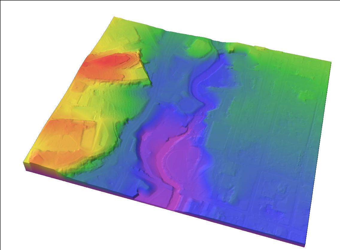

Close-up view:

set_camerapos(fig_nosinks, sc_nosinks, view2...)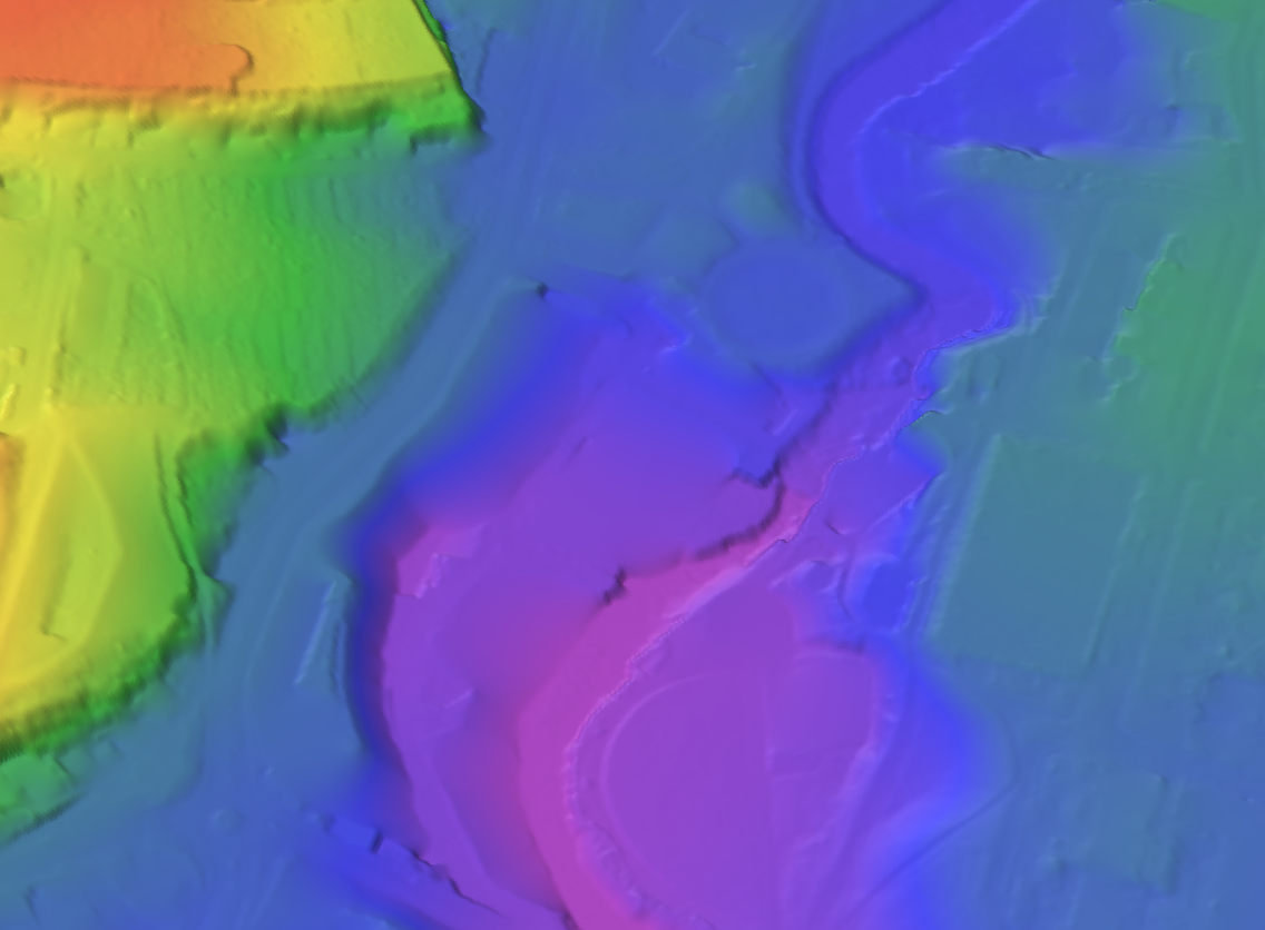

With sinks:

With manholes and other sinks, the submerged part of the terrain is significantly reduced, and the road is not flooded. In this analysis, infiltration has not yet been considered. Many backyards are still under water.

sf_sinks, fig_sinks, sc_sinks = plotgrid(grid_dtm, texture=overlay_sinks);

fig_sinks
set_camerapos(fig_sinks, sc_sinks, view1...)

Close-up view:

set_camerapos(fig_sinks, sc_sinks, view2...)

Visualize flow intensity

The flow intensity at each given point in the terrain depends on the upstream area draining into that point, and how much rain is currently hitting that area. This also depends on whether upstream lakes have been filled yet or not. To analyze this, the watercourses function can be used. In addition to the terrain analysis data, the function takes precipitation and infiltration rates as input, as well as a vector indicating the lakes that are currently filled and spilling over. It returns a field showing the flow intensity field over the whole domain.

In the call to watercourses below, the unit used when specifying precipitation and infiltration (e.g. mm/hour, which translates into volume/time for a cell with finite area) will also determine the unit used for describing flow intensity (volume per time passing through the cell).

# assume all traps already filled
filled_traps = fill(false, numtraps(tstruct_sinks))

# compute flow intensity on terrain
precip = fill(1.0, size(tstruct_sinks.topography)...) # uniform precipitation field
infil = fill(0.0, size(tstruct_sinks.topography)...) # zero infiltration
runoff, = watercourses(tstruct_sinks, filled_traps,
                       precipitation=precip, infiltration=infil);

The result can be visualized using plotgrid:

# Plot runoff as a texture on the terrain, using a predefined colormap:
sf_flow, fig_flow, sc_flow =
    plotgrid(grid_dtm, texture=runoff,
             colormap=:Blues)
fig_flow
set_camerapos(fig_flow, sc_flow, view1...)

# Close-up view:
set_camerapos(fig_flow, sc_flow, view2...)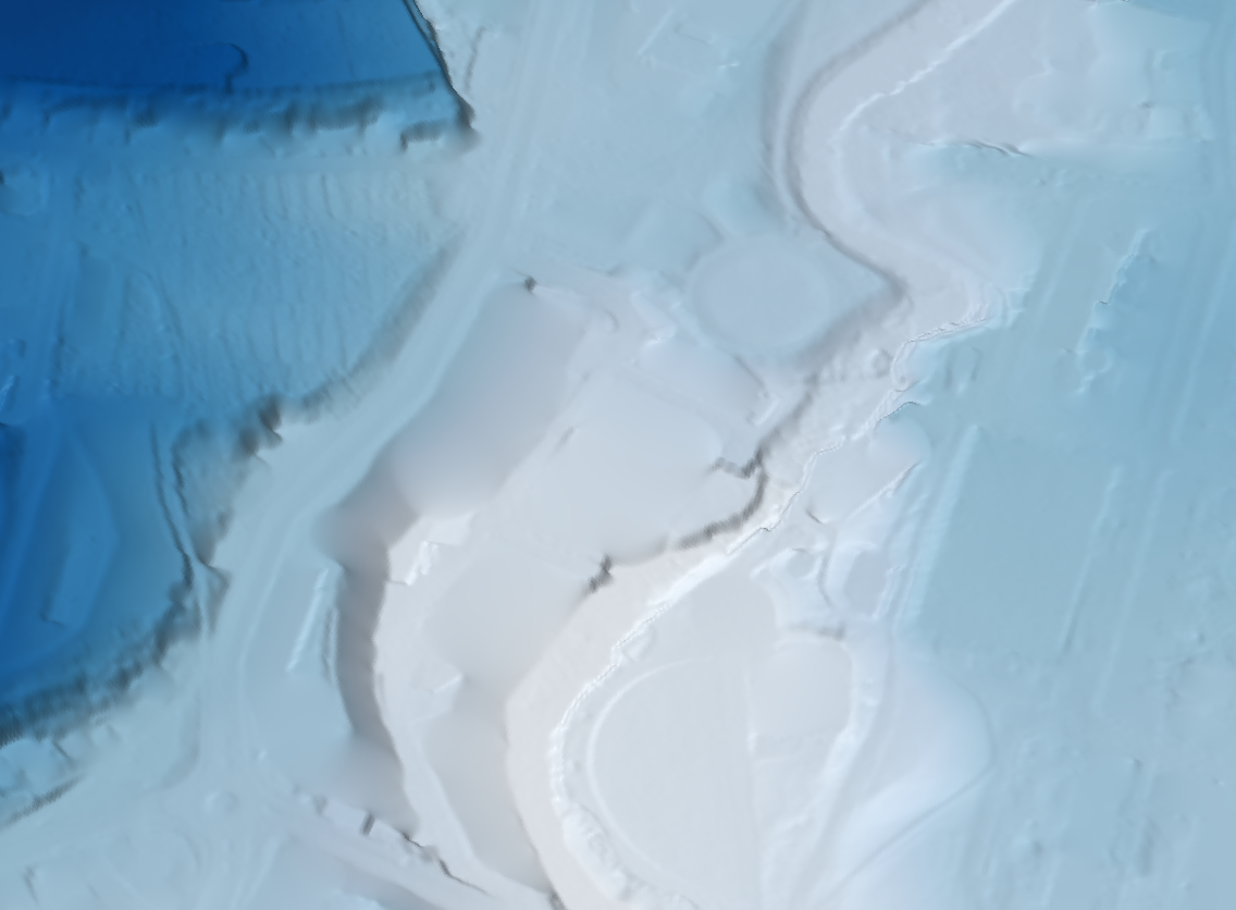

Only a few spots are colored non-white in the above plots. This is because the flow across the terrain is highly concentrated in a few locations with strong intermittent streams, where the flow values are much higher than elsewhere. If we want to highlight also the smaller flow patterns, a logarithmic scale can be useful:

sf_flow_log, fig_flow_log, sc_flow_log =
    plotgrid(grid_dtm, texture=log10.(runoff), colormap=:Blues)

fig_flow_log
set_camerapos(fig_flow_log, sc_flow_log, view1...)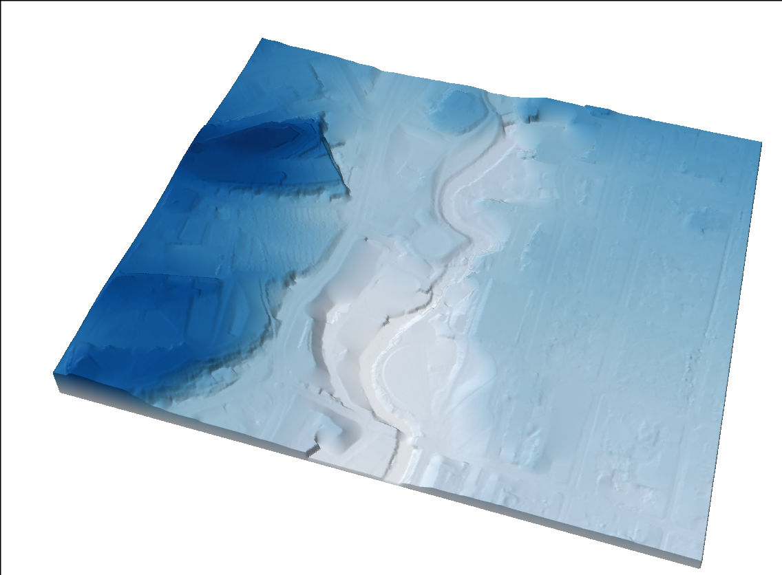

Close-up view:

set_camerapos(fig_flow_log, sc_flow_log, view2...)

On these logarithmic plots, differences between strong and weak flows are attenuated, and it is easier to see how the water flows.

Visualize upstream areas

The flow intensity map is useful to identify the areas with high flowrate, but does not indicate the origin of the flow. The upstream_area function can be used to determine the complete upstream watershed associated with any given cell in the terrain grid. To demonstrate its use, we select a gridcell with high flow rate, and use upstream_area to identify its upstream region.

max_runoff = extrema(runoff)[2] # the maximum flow value found in the grid
pt = findall(runoff .== max_runoff) # identify the corresponding cell
pt_ix = LinearIndices(grid_dtm)[pt[1]] # convert `pt` (a `CartesianIndex`) to linear index

# Identify cells belonging to the upstream area of `pt`, upsample to twice
# the grid resolution (to match the resolution of the map texture), and
# overwrite it on a copy of the map texture using blue color.
upstream_cells = upstream_area(tstruct_sinks, pt_ix, local_only=false)
tmp_ind = fill(false, size(grid_dtm))
tmp_ind[upstream_cells] .= true
tmp_ind = doublesize(tmp_ind);
upstream_texture = copy(mapimg)
upstream_texture[tmp_ind] = 0.5 * blue_color .+ 0.5 .* mapimg[tmp_ind]

# Identify the point `pt` itself in the grid.  We need to upsample this point too.
tmp_ind = fill(false, size(grid_dtm))
tmp_ind[pt_ix] = true
tmp_ind = doublesize(tmp_ind)
pt_ix_upscaled = findall(tmp_ind)

# Flag sink locations in black and the point `pt` in red
sink_locs = findall(sink_mask .> Images.Gray(0.0))
upstream_texture[sink_locs] .= black_color
upstream_texture[pt_ix_upscaled] .= red_color

# Plot the grid
sf_upstr_log, fig_upstr_log, sc_upstr_log = plotgrid(grid_dtm, texture=upstream_texture)

fig_upstr_log
set_camerapos(fig_upstr_log, sc_upstr_log,
              CairoMakie.Vec(-17, 202, 178), # observer position
              CairoMakie.Vec(472, 113, -255), # observer target
              0.8)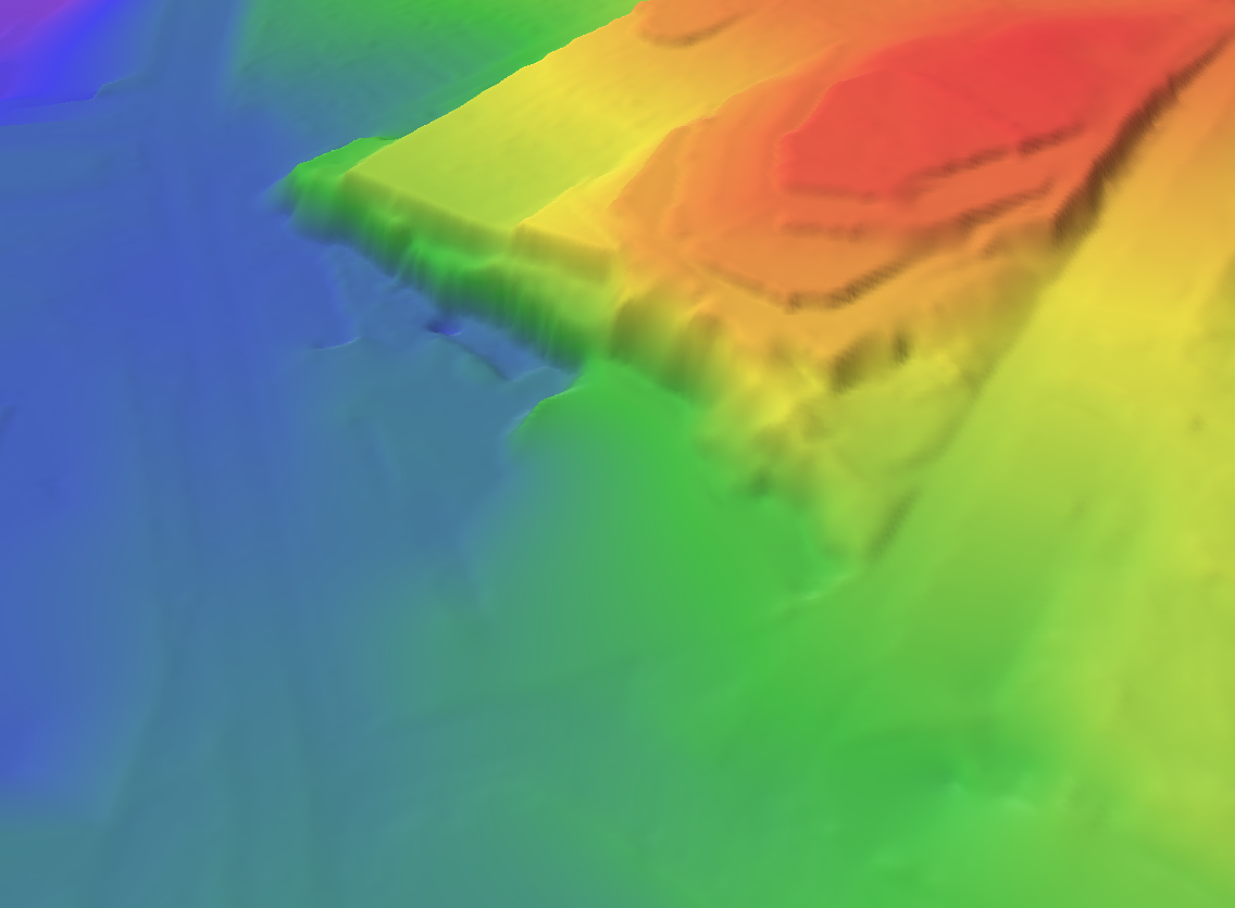

The point pt can be seen in red on the lower left part of this image, and all the black gricells indicate the position of sinks. The upstream area of pt is indicated with the blue color. The "holes" in this upstream area are caused by the associated sinks. All the water that falls on the blue are will pass through the point pt.

Infiltration and temporal development

A purely static analysis cannot properly capture the temporal aspect of infiltration. On terrains with permeable surfaces, evaluating whether or not an area gets flooded involves looking at the balance of inflow and infiltration as it develops over time.

Currently, SWIM includes a simplified infiltration model, where infiltration rates depends on spatial location, but remains constant over a defined time interval^[2]. By specifying the precipitation intensity (which may vary in space and time), a sequence of events may be computed that shows how terrain fills up, drains or equilbrates over time.

Below, we demonstrate the sequence computation on the terrain twice: first without considering infiltration, then by considering certain parts of terrain permeable with a specified drainage rate.

We first define a vector of WeatherEvents. These events indicate points in time when the weather changes. For example, using two events, we can designate a time where rain with a given rate starts and stops. Rain rates can be specified as a single number for the whole domain, or as a map of values over the terrain.

To keep things simple in this demonstration, our "weather" vector consists of a single event, where rain starts at hour 0.0, at a uniform rate of 20mm/h across the whole domain.

weather = [WeatherEvent(0.0, 20 * 1e-3),]

1-element Vector{WeatherEvent}:
 WeatherEvent(0.0, 0.02)

For the case with infiltration, we use the precipitation mask, resize it to the grid resolution, convert it to Bool, and multiply it with the infiltration value (25 mm/h). Note that we here use an infiltration value that is higher than the prescribed rain rate (20mm/h), so areas with will need influx of water from upstream to start filling up.

pmask = Images.imresize(permeable_mask, size(grid_dtm))
pmask[pmask .!= Images.Gray{Images.N0f8}(0.0)] .= Images.Gray{Images.N0f8}(1.0)
pmask = Matrix{Bool}(pmask .== Images.Gray{Images.N0f8}(1.0));
infil = 25.0 * 1e-3 * pmask;

We use the result of our static trap analysis with sinks to compute the time sequence. In other words, the city drainage system is here considered able to evacuate all water that enters manholes, etc.

seq1 = fill_sequence(tstruct_sinks, weather) # result with no infiltration
seq2 = fill_sequence(tstruct_sinks, weather, infiltration=infil); # result with infiltration

By looking at the timestamp for the last event in the sequence, we can assess the time it takes in the two cases before steady state is reached (i.e. all traps filled up, or reached equilibrium).

(seq1[end].timestamp, seq2[end].timestamp)

(36.92735528887271, 132.1674412590167)

Without infiltration, the end state is here reached in 37 hours, whereas it takes more than 132 hours when infiltration is included.

Visualize time sequence

Using the generated sequence of events, we can visualize the gradual accumulation (or depletion) of water on the terrain by creating a series of "snapshot" textures at specified timepoints, and then draping them over the terrain in the viewer.

First, we create a texture that we will use as background image when drawing the updates. For this, we use map image, and paint the river blue. As we will visualize two cases, we make two copies of this texture.

animated_overlay_1 = copy(mapimg);
animated_overlay_1[river_mask .> Images.Gray{Images.N0f8}(0.0)] .= blue_color;
animated_overlay_2 = copy(animated_overlay_1)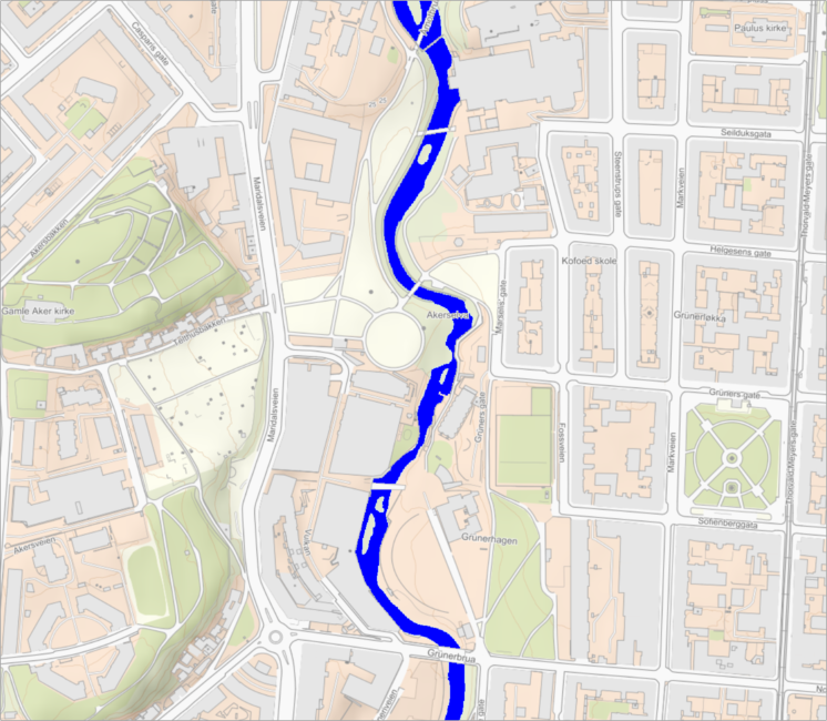

We now specify the time steps for which we want to visualize the state of the terrain. Since the most rapid and interesting changes happen early, we here visualize the first two hours. We compute 100 textures, equidistant in time.

t_end = 2.0 # specify the time at the end of the visualized period (2 hours)
timepoints = collect(range(0.0, t_end, length=100)); # specify the timepoints

The function interpolate_timeseries is used to compute the 100 textures. Since the returned textures have the resolution of the grid, whereas we want to superimpose them on the animated_overlay texture which has twice the resolution, we reuse the doublesize function that we defined earlier:

series1, = interpolate_timeseries(tstruct_sinks, seq1, timepoints, verbose=false)
series2, = interpolate_timeseries(tstruct_sinks, seq2, timepoints, verbose=false)

# The following code block plots the 3D grid and then
surface1, f1, sc1 = plotgrid(grid_dtm, texture = animated_overlay_1)
surface2, f2, sc2 = plotgrid(grid_dtm, texture = animated_overlay_2)

for i = 1:length(timepoints)
    s1, s2 = doublesize(series1[i]), doublesize(series2[i])

    # filled part of traps
    animated_overlay_1[s1[:] .== 1] .= blue_color
    animated_overlay_2[s2[:] .== 1] .= blue_color

    # rivers
    animated_overlay_1[s1[:] .== 3] .= blue_color
    animated_overlay_2[s2[:] .== 3] .= blue_color

    # Parts of lakes that are still not submerged
    animated_overlay_1[s1[:] .== 2] = 0.5 * mapimg[s1[:] .== 2] .+ 0.5 .* beige_color;
    animated_overlay_2[s2[:] .== 2] = 0.5 * mapimg[s2[:] .== 2] .+ 0.5 .* beige_color;

    # update textures on surfaces
    drape_surface(surface1, animated_overlay_1)
    drape_surface(surface2, animated_overlay_2)

    # brief pause
    sleep(0.05)
end

Although the animation above can not be shown directly in the online documentation, we can show the end states. To better see the differences, we use closeup views:

f1
set_camerapos(f1, sc1, vie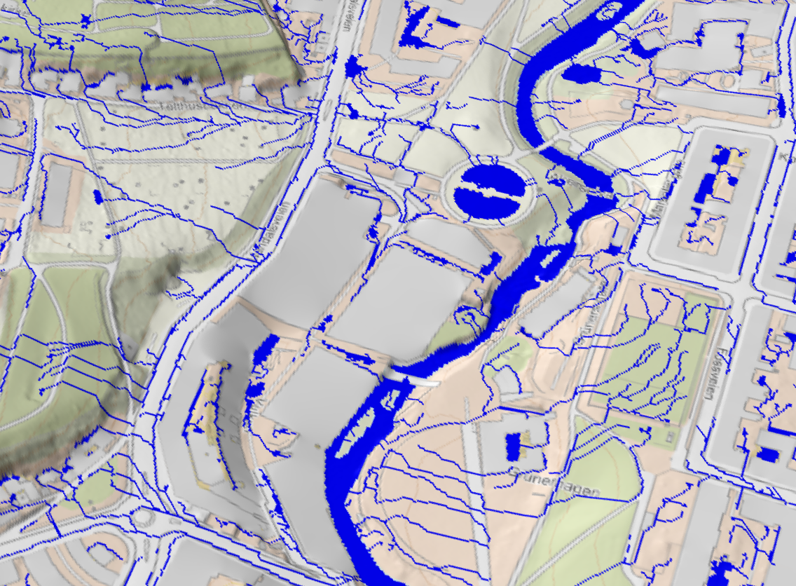w2...)

Terrain state at end of animated period, assuming no infiltration.

f2
set_camerapos(f2, sc2, vie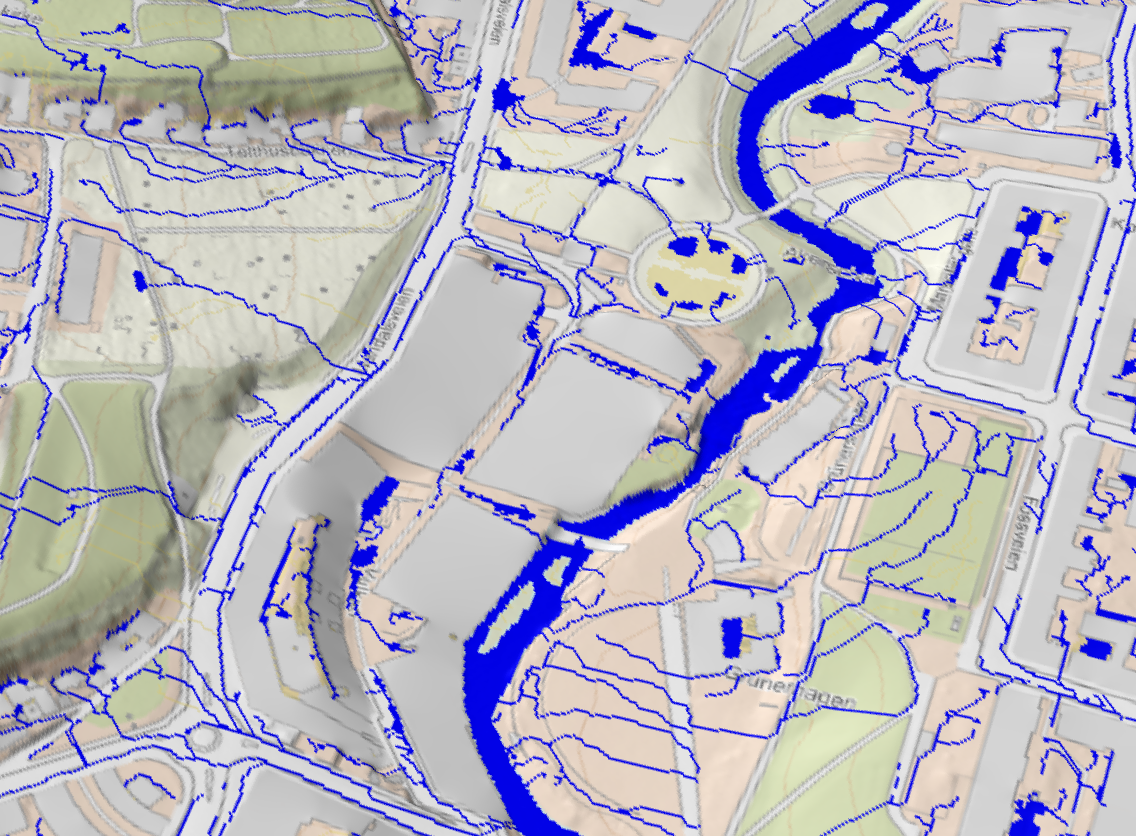w2...)

Terrain state at end of animated period, including the effect of infiltration.

Conclusion

At this point we conclude this demonstration of some main elements of SWIM:

Loading and preparation of data
Static analysis (identification of trap hierarchies and flow patterns, for a given surface, infrastructure and sinks)
Using the result of static analysis to visualize flow patterns and identify upstream areas.
Infiltration and simulating temporal developments.

This page was generated using Literate.jl.

1The data used in this example was originally obtained from Kartverket (the Norwegian Mapping Authority) under the Creative Commons Attribution 4.0 International (CC BY 4.0) license.
2This assumption may be relaxed by introducing new, updated infiltration rates at fixed points in time.