History matching of simulation models
We demonstrate history matching of a Direct Column Breakthrough (DCB) simulation model in Mocca. We leverage the powerful and flexible optimization functionality of Jutul to set up and perform the history matching. For more details about the DCB modelling, see the Simulate DCB example.
Import necessary modules
import Jutul
import Mocca
We create a function for setting up new simulation cases from the value of the parameter we wish to tune
function setup_case(prm, step_info=missing)

    param_dict_symb = Dict(Symbol(k) => v for (k, v) in prm);
    RealT = valtype(param_dict_symb);
    constants, info = Mocca.parse_input(Mocca.haghpanah_DCB_input(); typeT=RealT)

    for (k, v) in param_dict_symb
        print(k)
        print(v)
        setproperty!(constants, Symbol(k), v)
    end
    case,  = Mocca.setup_mocca_case(constants, info)

    return case
end;
Create synthetic reference data
constants_ref, = Mocca.parse_input(Mocca.haghpanah_DCB_input(); typeT=Float64)

prm_ref = Dict("v_feed" => constants_ref.v_feed);
case_ref = setup_case(prm_ref);v_feed0.37Configure simulator which will be used in the history matching
timestep_selector_cfg = (y=0.01, Temperature=10.0, Pressure=10.0)
sim, cfg = Mocca.setup_process_simulator(case_ref.model, case_ref.state0, case_ref.parameters;
    timestep_selector_cfg = timestep_selector_cfg,
    initial_dt = 1.0,
    output_substates = true,
    info_level = -1
);
Run reference simulation to generate and generate "ground truth" data from the result
states, timesteps_out = Mocca.simulate_process(case_ref;
    simulator = sim,
    config = cfg
);

times_ref = cumsum(timesteps_out)
total_time = times_ref[end]
last_cell_idx = Jutul.number_of_cells(case_ref.model.domain)
qCO2_ref = map(s -> getindex(s[:AdsorbedConcentration], 1, last_cell_idx), states)
qCO2_ref_by_time = Jutul.get_1d_interpolator(times_ref, qCO2_ref);
Setting up and solving the optimization problem
We define a suitable objective function to quantify the match between our simulations and the reference solution. Here we choose deviation of adsorbed CO2 in the last grid cell.
function objective_function(model, state, dt, step_info, forces)
    current_time = step_info[:time]
    q_co2 = getindex(state[:AdsorbedConcentration], 1, last_cell_idx)
    q_co2_ref = qCO2_ref_by_time(current_time)
    v = dt/total_time*(q_co2 - q_co2_ref)^2
    return v
end;
Perturb the known parameter $v_{feed}$ to form our initial guess for the optimization
prm_guess = Dict("v_feed" => constants_ref.v_feed+0.2);Activate $v_{feed}$ as a free parameter
dprm = Jutul.DictOptimization.DictParameters(prm_guess)
Jutul.DictOptimization.free_optimization_parameter!(dprm, "v_feed"; rel_min = 0.001, rel_max = 100.0)
DictParameters with 1 parameters (1 active), and 0 multipliers:
Active optimization parameters
┌────────┬───────────────┬───────┬─────────┬──────┐
│ Name │ Initial value │ Count │ Min │ Max │
├────────┼───────────────┼───────┼─────────┼──────┤
│ v_feed │ 0.57 │ 1 │ 0.00057 │ 57.0 │
└────────┴───────────────┴───────┴─────────┴──────┘
No inactive optimization parameters.
No multipliers set.
Run the optimization
prm_opt = Jutul.DictOptimization.optimize(dprm, objective_function, setup_case;
    config = cfg,
    max_it = 10,
    obj_change_tol = 1e-6,
    solution_history = true
);
Optimization: Starting calibration of 1 parameters.
Optimization: Setting up adjoint storage.
Optimization: Finished setup in 6.193797328 seconds.
Optimization: Adjoint solve took 3.812714225 seconds.
Optimization: Objective #1: 7.61286e+05, gradient 2-norm: 4.71893e+06
It. | Objective | Proj. grad | Linesearch-its
-----------------------------------------------
0 | 1.6133e-01 | 5.6999e+01 | -
Optimization: Adjoint solve took 0.257879584 seconds.
Optimization: Objective #2: 6.36994e+06 (f/f0=8.367e+00), gradient 2-norm: 1.21894e-04
Optimization: Adjoint solve took 3.034660481 seconds.
Optimization: Objective #3: 6.05491e+05 (f/f0=7.954e-01), gradient 2-norm: 5.00075e+06
Optimization: Adjoint solve took 3.439609487 seconds.
Optimization: Objective #4: 1.24529e+06 (f/f0=1.636e+00), gradient 2-norm: 6.30573e+06
Optimization: Adjoint solve took 2.985546101 seconds.
Optimization: Objective #5: 1.60276e+05 (f/f0=2.105e-01), gradient 2-norm: 4.25403e+06
Optimization: Adjoint solve took 0.245650385 seconds.
Optimization: Objective #6: 6.36994e+06 (f/f0=8.367e+00), gradient 2-norm: 1.21894e-04
LBFGS: Line search unable to succeed in 5 iterations ...
Optimization: Adjoint solve took 3.001294302 seconds.
Optimization: Objective #7: 1.60276e+05 (f/f0=2.105e-01), gradient 2-norm: 4.25403e+06
LBFGS: Resetting 'm' to number of parameters: m = 1
1 | 3.3964e-02 | 5.6999e+01 | 5
Optimization: Adjoint solve took 0.250155374 seconds.
Optimization: Objective #8: 6.36994e+06 (f/f0=8.367e+00), gradient 2-norm: 1.21894e-04
Optimization: Adjoint solve took 2.999746663 seconds.
Optimization: Objective #9: 9.17200e+04 (f/f0=1.205e-01), gradient 2-norm: 3.55824e+06
2 | 1.9437e-02 | 5.1384e+01 | 2
Optimization: Adjoint solve took 3.083882304 seconds.
Optimization: Objective #10: 1.56515e+05 (f/f0=2.056e-01), gradient 2-norm: 6.37615e+06
Optimization: Adjoint solve took 2.954926263 seconds.
Optimization: Objective #11: 5.98917e+01 (f/f0=7.867e-05), gradient 2-norm: 1.18220e+05
3 | 1.2692e-05 | 4.2980e+01 | 2
Optimization: Adjoint solve took 2.963269522 seconds.
Optimization: Objective #12: 1.30250e+01 (f/f0=1.711e-05), gradient 2-norm: 4.91360e+04
4 | 2.7602e-06 | 1.4280e+00 | 1
Optimization: Adjoint solve took 2.990070626 seconds.
Optimization: Objective #13: 4.89064e-01 (f/f0=6.424e-07), gradient 2-norm: 1.02865e+04
5 | 1.0364e-07 | 5.9351e-01 | 1
Optimization: Adjoint solve took 3.023212934 seconds.
Optimization: Objective #14: 1.31567e-02 (f/f0=1.728e-08), gradient 2-norm: 1.63327e+03
6 | 2.7881e-09 | 1.2425e-01 | 1
Optimization: Finished in 61.217479035 seconds.We can see a clear reduction of the objective function value throughout the optimization iterations, indicating a close match between the reference solution and our simulation.
f = Mocca.plot_optimization_history(dprm)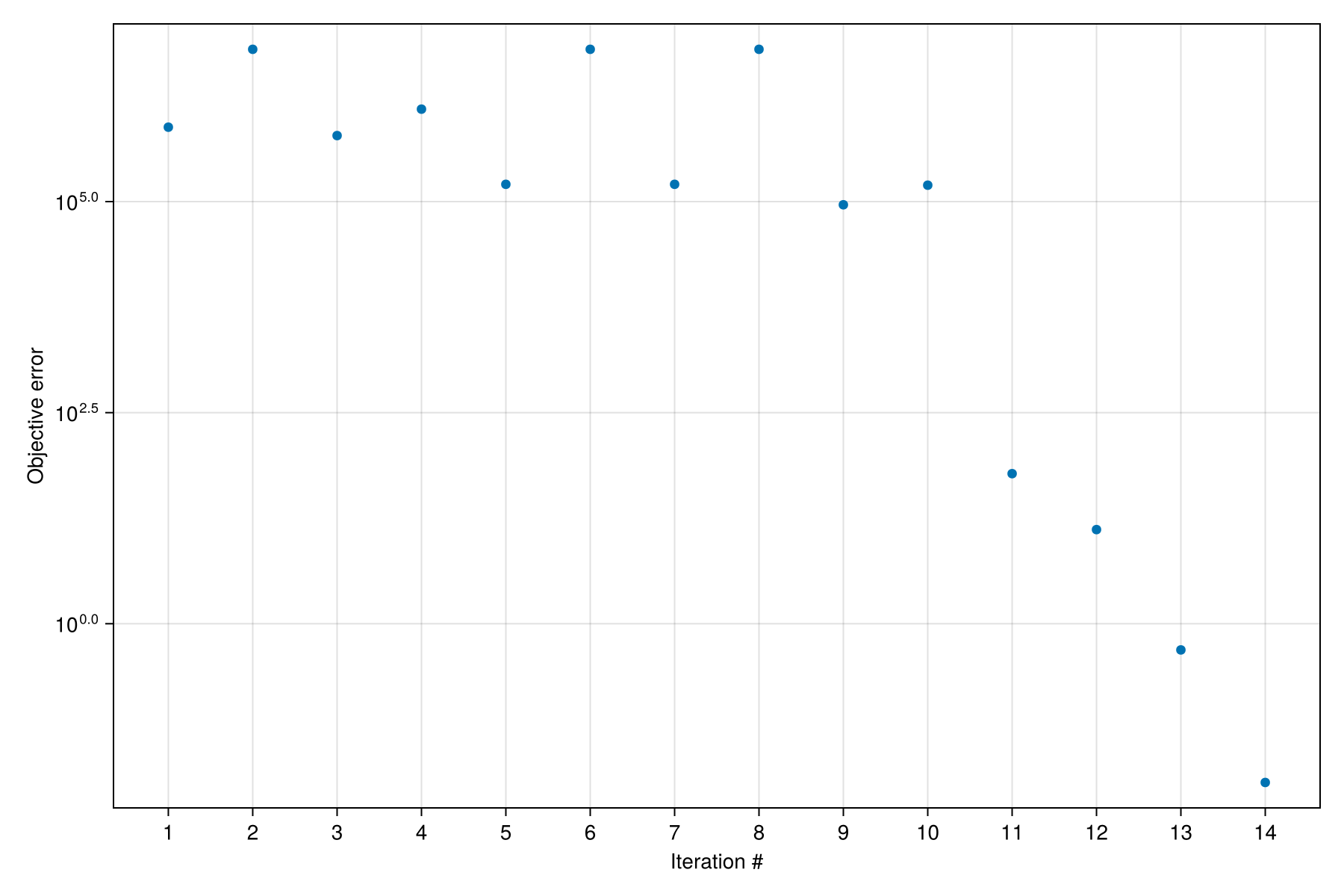
We can look at the optimization result:
dprmDictParameters with 1 parameters (1 active), and 0 multipliers:
Active optimization parameters
┌────────┬───────────────┬───────┬─────────┬──────┬─────────────────┬────────┐
│ Name │ Initial value │ Count │ Min │ Max │ Optimized value │ Change │
├────────┼───────────────┼───────┼─────────┼──────┼─────────────────┼────────┤
│ v_feed │ 0.57 │ 1 │ 0.00057 │ 57.0 │ 0.37 │ -35.0% │
└────────┴───────────────┴───────┴─────────┴──────┴─────────────────┴────────┘
No inactive optimization parameters.
No multipliers set.
and see that the value matches the reference parameter value
constants_ref.v_feed0.37Check size of objective mismatch
dprm.history.objectives14-element Vector{Float64}:
761285.8833491696
6.369944548281407e6
605490.5988767222
1.2452850490274746e6
160276.16543350072
6.369944548281407e6
160276.16543350072
6.369944548281407e6
91720.04717463219
156514.61420140337
59.8916510935571
13.024970005004135
0.48906387349270003
0.013156736829874468Example on GitHub
If you would like to run this example yourself, it can be downloaded from the Mocca.jl GitHub repository.
This page was generated using Literate.jl.