Cyclic Vacuum Swing Adsorption simulation
This example shows how to set up and run a cyclic vacuum swing adsorption simulation as described in Haghpanah et al. 2013
This simulation inolves injection of a two component flue gas (CO2 and N2) into a column of Zeolite 13X. The CO2 is preferentially adsorbed onto the zeolite. Pressure in the column is then reduced to enable desorption of CO2 for collection.
This is a four stage process comprising:
- Pressurisation: Where the RHS of the column is closed and flue gas is injected from the LHS, at velocity $v_{feed}$, to bring the column pressure up to $P_H$ (Pressure High).
- Adsorption: Where both ends of the column are open and flue gas is injected from the RHS at velocity $v_{feed}$. Pressure at the LHS is $P_H$.
- Blowdown: Where the LHS of the column is closed and the column is evacuated at $P_I$ (Pressure Intermediate).
- Evacuation: Where the RHS of the column is closed and the column is evacuated from the LHS at $P_L$ (Pressure Low).
Each stage is modelled using the same governing equations but with different boundary conditions. Adsorption onto Zeolite 13X is modelled with a dual-site Langmuir adsorption isotherm.
First we load the necessary modules
import Jutul
import Jutul: si_unit
import Mocca
We define parameters, and set up the system and domain as in the Haghpanah DCB example.
constants = Mocca.HaghpanahConstants{Float64}()
system = Mocca.AdsorptionSystem(constants);
Create the model
Now we can assemble the model which contains the domain and the system of equations.
ncells = 200
model = Mocca.setup_process_model(system, constants; ncells = ncells);
Setup the initial state and parameters
Initial values for pressure and temperature of the system
bar = si_unit(:bar);
P_init = 1*bar;
T_init = 298.15;
Tw_init = constants.T_a;
To avoid numerical errors we set the initial CO2 concentration to be very small and not exactly zero
yCO2_2 = 1e-10
y_init = [yCO2_2, 1.0 - yCO2_2] # [CO2, N2]

state0 = Mocca.setup_process_state(model;
    Pressure = P_init,
    Temperature = T_init,
    WallTemperature = Tw_init,
    y = y_init
);

parameters = Mocca.setup_process_parameters(model);
Set up the stage timings and boundary conditions
Here we have 4 stages and we specify a duration in seconds that we will run each stage.
t_press = 15.0
t_ads = 15.0
t_blow = 30.0
t_evac= 40.0
stage_times = [t_press, t_ads, t_blow, t_evac];
stage_names = ["pressurisation", "adsorption", "blowdown", "evacuation"]
bcs = Mocca.setup_boundary_conditions(constants, stage_names)
4-element Vector{Any}:
Mocca.PressurisationBC{Float64, 2}
y_feed: StaticArraysCore.SVector{2, Float64}
PH: Float64 100000.0
PL: Float64 10000.0
λ: Float64 0.5
T_feed: Float64 298.15
stage_start: Float64 0.0
Mocca.AdsorptionBC{Float64, 2}
y_feed: StaticArraysCore.SVector{2, Float64}
PH: Float64 100000.0
v_feed: Float64 0.37
T_feed: Float64 298.15
Mocca.BlowdownBC{Float64}
PH: Float64 100000.0
PI: Float64 20000.0
λ: Float64 0.5
stage_start: Float64 0.0
Mocca.EvacuationBC{Float64}
PL: Float64 10000.0
PI: Float64 20000.0
λ: Float64 0.5
stage_start: Float64 0.0
Set up cyclic boundary conditions and timesteps for the simulation We will run 3 cycles of the process for demonstration purposes, to reach steady state num_cycles should be increased.
sim_forces, timesteps = Mocca.setup_forces(model, stage_times, bcs;
    num_cycles=3, max_dt = 1);
Simulate
Now we are ready to run the simulation
case = Mocca.MoccaCase(model, timesteps, sim_forces; state0 = state0, parameters = parameters)
states, timesteps_out = Mocca.simulate_process(case;
    output_substates = true,
    info_level = 0
);
Jutul: Simulating 5 minutes as 300 report steps
╭────────────────┬───────────┬───────────────┬───────────╮
│ Iteration type │ Avg/step │ Avg/ministep │ Total │
│ │ 300 steps │ 304 ministeps │ (wasted) │
├────────────────┼───────────┼───────────────┼───────────┤
│ Newton │ 2.65 │ 2.61513 │ 795 (30) │
│ Linearization │ 3.66333 │ 3.61513 │ 1099 (32) │
│ Linear solver │ 2.65 │ 2.61513 │ 795 (30) │
│ Precond apply │ 0.0 │ 0.0 │ 0 (0) │
╰────────────────┴───────────┴───────────────┴───────────╯
╭───────────────┬────────┬────────────┬────────╮
│ Timing type │ Each │ Relative │ Total │
│ │ ms │ Percentage │ s │
├───────────────┼────────┼────────────┼────────┤
│ Properties │ 1.2272 │ 30.75 % │ 0.9756 │
│ Equations │ 0.6253 │ 21.66 % │ 0.6872 │
│ Assembly │ 0.0293 │ 1.02 % │ 0.0322 │
│ Linear solve │ 1.7061 │ 42.75 % │ 1.3564 │
│ Linear setup │ 0.0000 │ 0.00 % │ 0.0000 │
│ Precond apply │ 0.0000 │ 0.00 % │ 0.0000 │
│ Update │ 0.0358 │ 0.90 % │ 0.0285 │
│ Convergence │ 0.0232 │ 0.80 % │ 0.0255 │
│ Input/Output │ 0.0367 │ 0.35 % │ 0.0112 │
│ Other │ 0.0707 │ 1.77 % │ 0.0562 │
├───────────────┼────────┼────────────┼────────┤
│ Total │ 3.9909 │ 100.00 % │ 3.1728 │
╰───────────────┴────────┴────────────┴────────╯Visualisation
We plot primary variables at the outlet through time
outlet_cell = ncells
f_outlet = Mocca.plot_cell(states, model, timesteps_out, outlet_cell)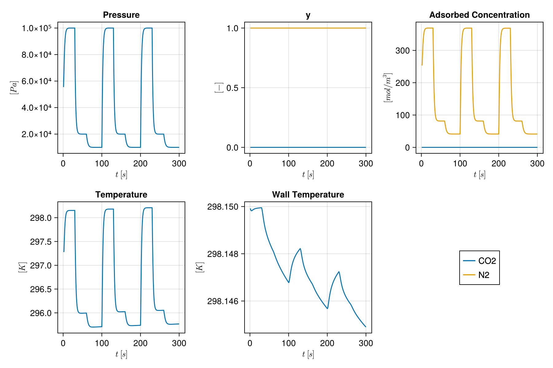
We also plot primary variables along the column at the end of the simulation
f_column = Mocca.plot_state(states[end], model)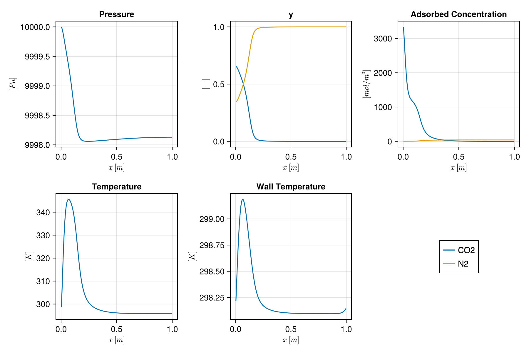
Example on GitHub
If you would like to run this example yourself, it can be downloaded from the Mocca.jl GitHub repository.
This page was generated using Literate.jl.