Jutul documentation
About
Jutul is an experimental Julia framework for multiphysics processes based on implicit finite-volume methods with automatic differentiation. The main public demonstrator is JutulDarcy.jl - a fully differentiable porous media simulator with excellent performance.
An example
Jutul is primarily intended to build applications. The base library includes a few "hello world"-type PDE solvers that are used for testing. One of these is the standard 2D heat equation on residual form:
$\frac{\partial T}{\partial t} - \frac{\partial^2 T}{\partial x^2} - \frac{\partial^2 T}{\partial y^2} = 0$
The test solver uses a structured grid and a central difference scheme with periodic boundary conditions to solve this system. You can view the complete source code for this solver here.
Simulation loop
We demonstrate how to set up the simulation loop. This essentially boils down to three things: Setting up a grid/model, setting initial condition and picking time-steps where the solver should report output:
using Jutul
sys = SimpleHeatSystem()
# Create a 100x100 grid
nx = ny = 100
L = 100.0
H = 100.0
g = CartesianMesh((nx, ny), (L, H))
# Create a data domain with geometry information
D = DataDomain(g)
# Set up a model with the grid and system
model = SimulationModel(D, sys)
# Initial condition is random values
nc = number_of_cells(g)
T0 = zeros(nc)
x = D[:cell_centroids][1, :]
y = D[:cell_centroids][2, :]
# Create initial peak of heat to diffuse out.
for i in 1:nc
    if (x[i] > 0.25*L) & (x[i] < 0.75*L) & (y[i] > 0.25*H) & (y[i] < 0.75*H)
        T0[i] = 100.0
    end
end
state0 = setup_state(model, Dict(:T=>T0))
sim = Simulator(model, state0 = state0)
dt = fill(1.0, 100)
states, = simulate(sim, dt, info_level = 1);
SimResult with 100 entries:
states (model variables)
:T => Vector{Float64} of size (10000,)
reports (timing/debug information)
:ministeps => Vector{Any} of size (1,)
:total_time => Float64
:output_time => Float64
Completed at Jul. 01 2026 18:13 after 5 seconds, 952 milliseconds, 271.7 microseconds.Visualizing the results
If using Julia 1.9 or later, visualization is provided if a version of Makie is included. In the documentation we use CairoMakie as it can produce plots on servers without rendering capabilities, such as the one where the Jutul continious integration is running:
using CairoMakieIf you are running this locally and want interactive plots you can instead use the GLMakie backend.
using GLMakie
GLMakie.activate!()
We plot the initial conditions:
fig, ax = plot_cell_data(g, state0[:T])
fig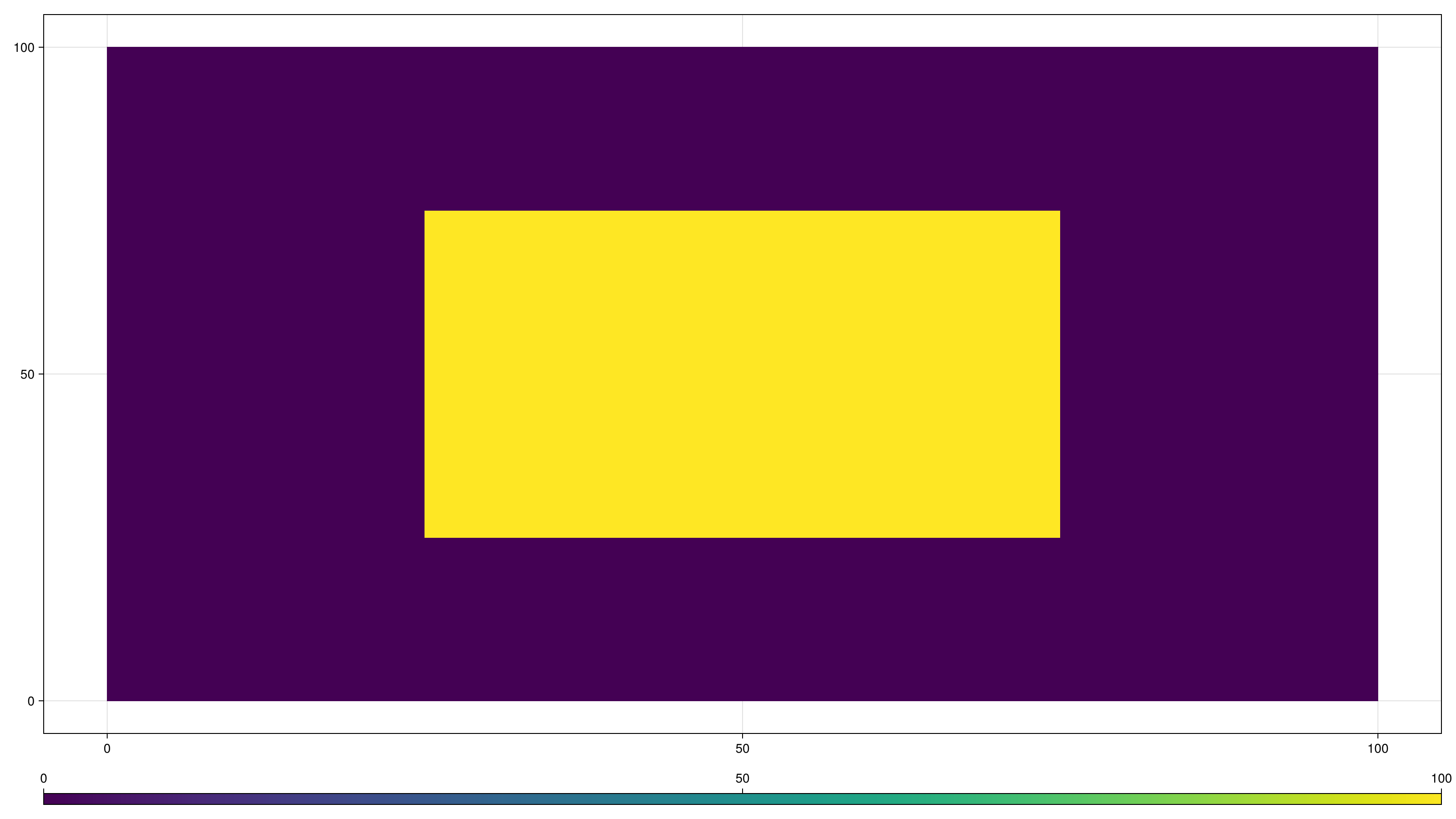
We can then plot the final state, observing significant diffusion from the sharp initial state.
fig, ax = plot_cell_data(g, states[end][:T])
fig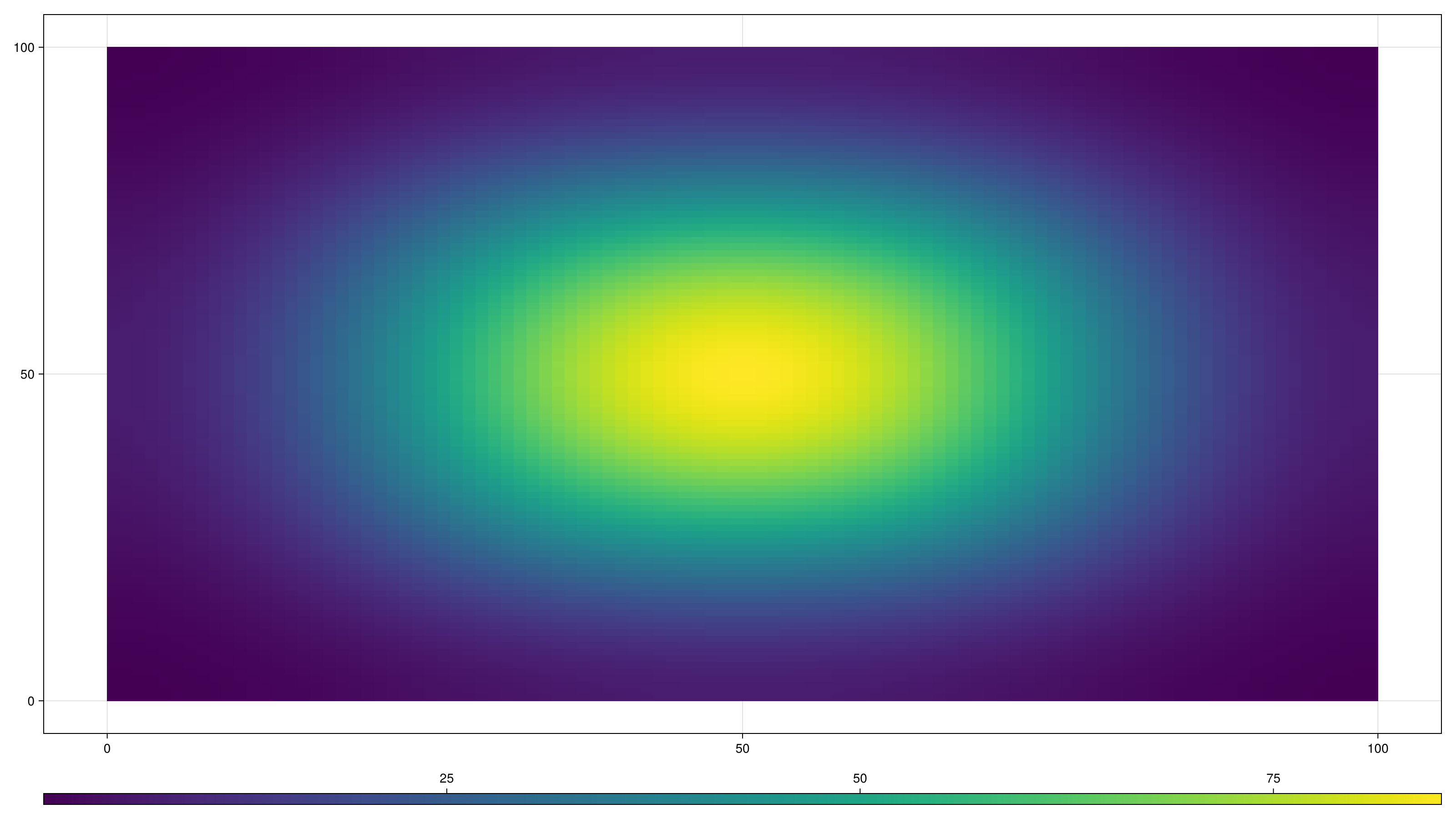
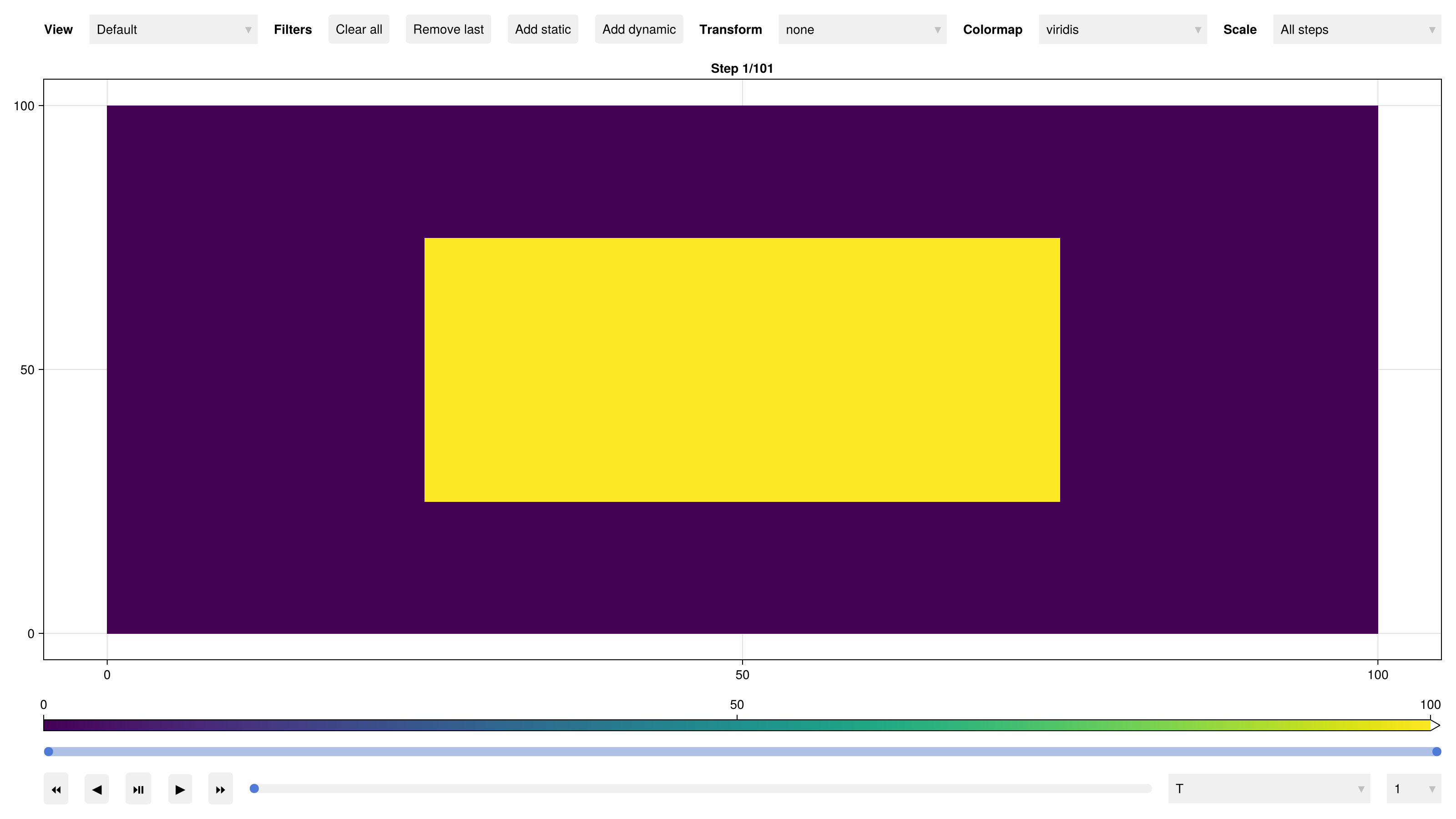
There is also interactive plotting that allows you to step through each time-step. This is most relevant when using GLMakie to plot, otherwise the figure will be static.
plot_interactive(g, [state0; states])